Introduction to Linear Algebra
Notes of the book Introduction to Linear Algebra.
$Ax$
Matrix multiplication $Ax$ can be viewed as using $x$ to form a linear combination of the columns of $A$.
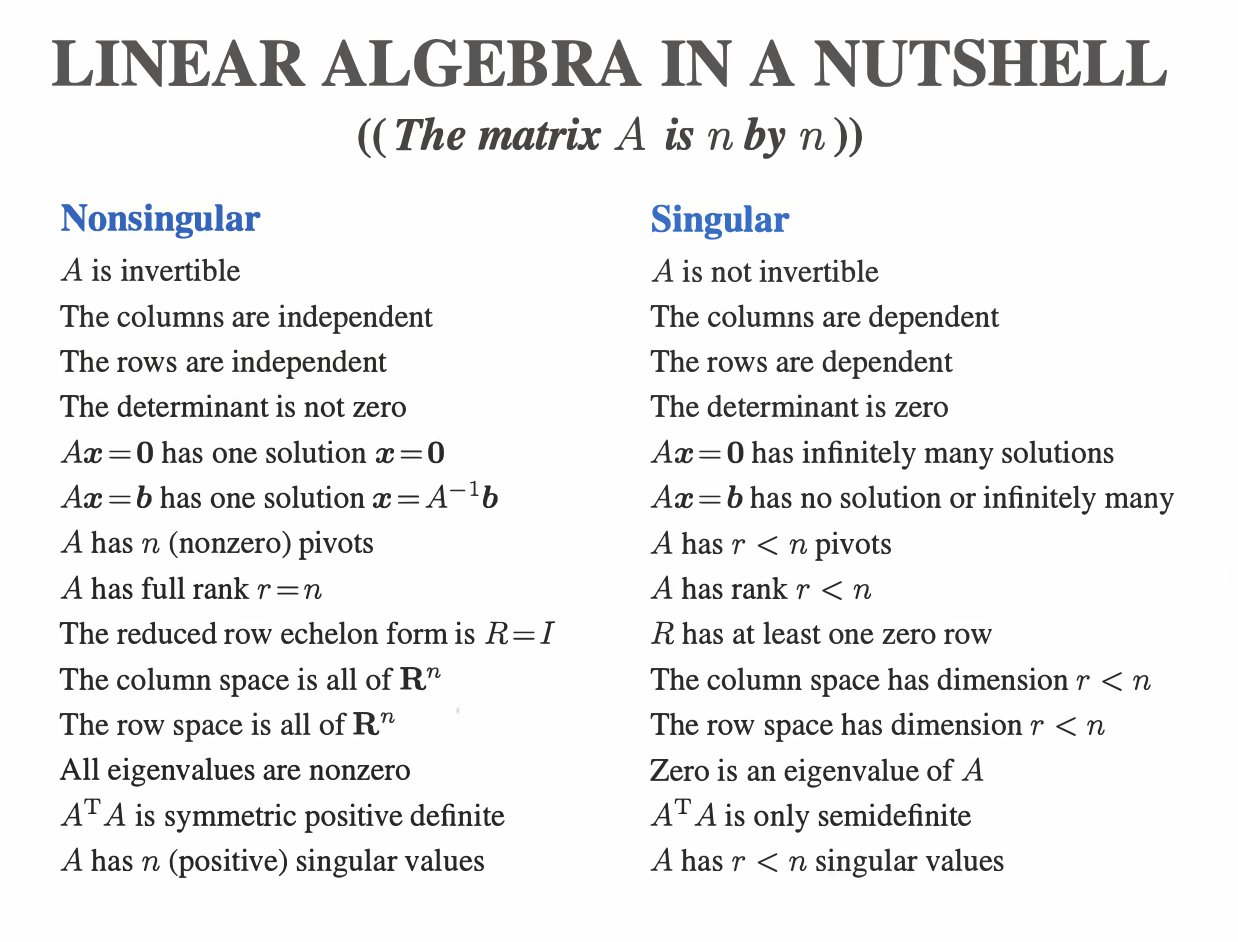
$Ax = 0$
- $x = 0$ is always a solution. The remaining solutions form the null space $N(A)$ of $A$, whose dimension (number of basis vectors) is $n - r$.
- For a tall (or square) $A$:
- If $A$ has full column rank (null space dimension 0), there is no nonzero solution.
- If $A$ does not have full column rank (null space has positive dimension), there are infinitely many nonzero solutions.
- For a wide $A$, there are always infinitely many nonzero solutions (the null space always has positive dimension).
$Ax = b$
- The taller $A$ is, the less likely it is to have a solution, since it is harder for the columns to span the whole $\mathbf{R}^m$ space.
- The wider $A$ is, the more likely it is to have a solution, since it is easier for the columns to span $\mathbf{R}^m$.
For the full-rank cases:
- Full row rank means there is always a solution (at least one):
- Every row has a pivot, so there is no zero row that would need to equal a nonzero entry of $b$.
- The number of solutions depends on whether $n - r$ is zero.
- Full column rank means the solution is unique (at most one):
- Every column has a pivot, so there are no free columns.
- The null space of $A$ has dimension $n - r = 0$.
In summary:
- Invertible square matrix ($m = n = r$): exactly one solution.
- Full-rank wide matrix: infinitely many solutions.
- Full-rank tall matrix: at most one solution.
- Neither full row rank nor full column rank: either no solution, or infinitely many, depending on whether a zero row happens to match a nonzero entry of $b$.
LU Factorization
$A = LU$
- A sequence of lower-triangular elimination matrices $E$ turns $A$ into the upper-triangular matrix $U$, i.e. $EA = U$.
- $U$ is the result of Gaussian elimination; each row/column has at most one pivot.
- $L$ is the inverse of the sequence of elimination operations $E$:
- $(E_n \dots E_2 E_1)^{-1} = L_1 L_2 \dots L_n = L$
- i.e. $L^{-1} A = U \Rightarrow A = LU$
- $L$ is itself lower triangular; each entry is the multiplier used during elimination.
- If row swaps are needed during the factorization, a permutation matrix $P$ is required (multiple $P$’s can be combined into one; the inverse of each $P$, and of the combined one, is $P^T$). The factorization then becomes $PA = LU$.
- Normalizing the pivots of $U$ to 1 gives $A = LDU$.
- For a symmetric $A$, we can write $A = LUL^T$, where the middle $U$ is a diagonal matrix of pivots.
- $U$ can be further reduced to $R$:
- Eliminate the entries above each pivot.
- Normalize each pivot to 1.
The Four Fundamental Subspaces of $A$
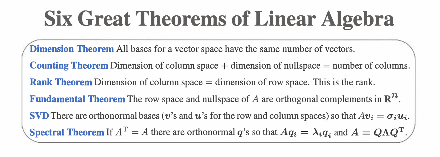
- The row space $C(A^T)$ has dimension $r$ and is a subspace of $\mathbf{R}^n$.
- It is spanned by the pivot rows of the final $R$ matrix.
- The null space $N(A)$ has dimension $n - r$ and is a subspace of $\mathbf{R}^n$ — the basis of the nonzero solutions of $Ax = 0$.
- It comes from the special solutions found via $R$.
- The column space $C(A)$ has dimension $r$ and is a subspace of $\mathbf{R}^m$.
- It is spanned by the columns of $A$ corresponding to the pivot columns of the final $R$ matrix.
- The left null space $N(A^T)$ has dimension $m - r$ and is a subspace of $\mathbf{R}^m$ — the basis of the nonzero solutions of $A^T x = 0$.
- It comes from the last $m - r$ rows of $E$ in $EA = R$.
$C(A^T)$ and $N(A)$ are orthogonal complements:
- Any vector from one space is orthogonal to any vector from the other.
- Together they span the whole $\mathbf{R}^n$ space.
- In other words: for a nonzero solution $x$ of $Ax = 0$, $x \in N(A)$ is orthogonal to every vector in the row space.
$C(A)$ and $N(A^T)$ are related the same way.
- If $A$ has full column rank, then $A^T A$ is always invertible, because $N(A) = {0}$ and $A^T A$ has the same null space as $A$, so $A^T A x = 0$ has no nonzero solution, i.e. $A^T A$ is invertible.
- $A$ maps a vector $x$ in $\mathbf{R}^n$ to $\mathbf{R}^m$.
Projections
- The projection of vector $b$ onto a line through point $a$ is the closest point on the line to $b$: $p = a \dfrac{a^T b}{a^T a}$.
- The projection of vector $b$ onto a subspace $S$ is the vector $p \in S$ such that $e = b - p$ is orthogonal to $S$.
- If $A$ has full column rank, the projection of $b$ onto the column space of $A$ is $p = A(A^T A)^{-1} A^T b$.
- The projection matrix is $P = A(A^T A)^{-1} A^T$, so $p = Pb$.
- When $Ax = b$ has no solution, we can find its least-squares solution:
- It minimizes $|b - Ax|^2$, i.e. it is the projection of $b$ onto the column space of $A$.
- It solves $A^T A x = A^T b$.
- Since $Ax = p = Pb$, we get $x = (A^T A)^{-1} A^T b$.
- QR factorization, $A = QR$:
- $Q$ is orthogonal ($Q^T Q = I$), $R$ is upper triangular.
- The factorization is obtained via Gram-Schmidt: the independent columns $a_i$ of $A$ are turned into an orthogonal basis $q_i$ through projection; $R$ stores the dot products between $Q$ and $A$.
- QR factorization lets us simplify $Ax = b$ into $Qy = b$, $Rx = y$, each of which is easy to solve.
Determinants
- The determinant can be computed in several ways:
- The “big formula” (sum over permutations).
- Cofactor expansion along the first row or first column.
- All properties of the determinant follow from three basic ones:
- The determinant of the identity matrix is 1.
- Swapping two rows negates the determinant.
- Multiplying one row by a scalar multiplies the determinant by that scalar.
Eigenvalues and Eigenvectors
$Ax = \lambda x$, where $A$ is a square matrix.
Some properties of eigenvalues:
- The sum of $A$’s eigenvalues equals $\text{trace}(A)$.
- The product of $A$’s eigenvalues equals $\det(A)$.
- $A^2$ has eigenvalues $\lambda^2$; $A^{-1}$ has eigenvalues $1/\lambda$; $A + I$ has eigenvalues $\lambda + 1$; $A^T$ has the same eigenvalues as $A$.
- Special cases:
- An orthogonal matrix has eigenvalues $1$ or $-1$, since $Q^{-1} = Q^T$.
- A projection matrix has eigenvalues $0$ or $1$, since $P^2 = P$.
- A reflection matrix has eigenvalues $1$ or $-1$.
- A diagonal/triangular matrix has its eigenvalues on the diagonal.
- If $A$ is not full rank (i.e. $\det(A) = 0$), then $0$ is one of its eigenvalues, since $Ax = 0$ has a nonzero solution.
- Similar matrices share the same eigenvalues.
- Repeatedly multiplying by $A$ eventually leaves only the eigenvector components with eigenvalue magnitude greater than 1.
For a square matrix $A$:
- Whether $0$ is an eigenvalue determines whether $A$ is invertible.
- Whether $A$ has repeated eigenvalues determines whether $A$ is diagonalizable:
- Eigenvectors for distinct eigenvalues are always independent.
- If all eigenvalues are distinct, all eigenvectors are independent, and $A$ is diagonalizable.
- If an eigenvalue is repeated, the number of independent eigenvectors for it is at most its multiplicity; $A$ is diagonalizable only if there are enough independent eigenvectors for every eigenvalue.
Diagonalization
- $A = X \Lambda X^{-1}$: using the (independent) eigenvector matrix to diagonalize $A$ into the eigenvalue matrix.
- Once diagonalized, computing high powers $A^k$ becomes easy.
Symmetric Matrices $S$
- A real symmetric matrix always has $n$ real eigenvalues (possibly repeated) and $n$ mutually orthogonal eigenvectors.
- $S = Q \Lambda Q^{-1} = Q \Lambda Q^T$
- The number of positive eigenvalues of $S$ equals the number of positive pivots.
- For a positive definite symmetric matrix:
- All pivots are positive.
- All eigenvalues are positive.
- All (leading) determinants are positive.
- $x^T S x > 0$ for every $x \neq 0$.
- $S = A^T A$ where all columns of $A$ are independent.
Singular Value Decomposition (SVD)
Every matrix $A$ can be factored as $A = U \Sigma V^T$.
- $\Sigma$ has $r$ (the rank of $A$) singular values on its diagonal, $\sigma_1 \geq \sigma_2 \geq \dots \geq \sigma_r > 0$. They are the square roots of the nonzero eigenvalues of $AA^T$ and $A^TA$.
- $AA^T$ and $A^TA$ are always positive (semi-)definite, i.e. all their eigenvalues are $\geq 0$.
- $x^T A^T A x = |Ax|^2 \geq 0$.
- $U$ consists of the orthogonal eigenvectors of $AA^T$: the first $r$ form a basis of $C(A)$, the remaining $m - r$ form a basis of $N(A^T)$.
- $V$ consists of the orthogonal eigenvectors of $A^TA$: the first $r$ form a basis of $C(A^T)$, the remaining $n - r$ form a basis of $N(A)$.
- $A = \sigma_1 u_1 v_1^T + \dots + \sigma_r u_r v_r^T$
- $A v_i = \sigma_i u_i$
Additional facts:
- The singular values of $A$ are the same as the eigenvalues of $\Sigma$, and are the square roots of the eigenvalues of $A^TA$ or $AA^T$.
- The closest matrix (of lower rank) to $A$ is obtained by setting the smallest singular value(s) in the SVD to 0.
- $|A| = \sigma_1$, the largest singular value, which is also the maximum of $|Ax| / |x|$.
- The pseudoinverse of $A$ is $A^+ = V \Sigma^+ U^T$, where $\Sigma^+$ takes the reciprocal of each nonzero entry of $\Sigma$.
- Since $A v_i = \sigma_i u_i$, $A$ maps:
- The row space $C(A^T)$ to the column space $C(A)$.
- The null space $N(A)$ to $0$.
- Since $A^+ u_i = \frac{1}{\sigma_i} v_i$, $A^+$ maps:
- The column space $C(A)$ to the row space $C(A^T)$.
- The left null space $N(A^T)$ to $0$.
- Since $A v_i = \sigma_i u_i$, $A$ maps:
Linear Transformations
- $T(cv + dw) = cT(v) + dT(w)$, so $T(0) = 0$.
- Every linear transformation can be represented by a matrix $A$:
- $T$ maps a vector $v$ in $\mathbf{R}^n$ (space $V$) to $\mathbf{R}^m$ (space $W$), so $A$ is $m \times n$.
- The value of $A$ depends on the chosen bases of $V$ and $W$, but all such matrices describe the same transformation.
- Mapping each basis vector $v_i$ of $V$ through $T$ and expressing $T(v_i)$ in the basis of $W$ gives the $i$-th column of $A$.
- Identity transformation: $T(v) = v$.
- It can be described by a square matrix $A$.
- If the standard basis is used, $A = I$.
- If $V$ and $W$ are used as the input and output bases respectively, $B = W^{-1}V$.
- For a general transformation with matching input/output dimensions (a square transformation matrix), with matrix $A$ in the standard basis:
- If $A$ has $n$ independent eigenvectors (i.e. is diagonalizable), choosing them as the basis $B$ for both input and output gives the transformation matrix $B^{-1}AB = \Lambda$, the eigenvalue matrix.
- If $A$ does not have $n$ independent eigenvectors, supplement them with extra vectors to form $B$. The transformation matrix becomes the Jordan normal form, with a $1$ above the diagonal entry for each supplemented vector.
- For a general transformation with different input/output dimensions, with matrix $A$ in the standard basis:
- Choose the right singular vectors $V$ as the input basis and the left singular vectors $U$ as the output basis.
- The resulting transformation matrix is $U^{-1}AV = \Sigma$, the (diagonal) singular value matrix.
Complex Matrices
- $z = a + bi = re^{i\theta}$, $\bar{z} = a - bi = re^{-i\theta}$
- $(a, b)$ can be viewed as a point in the 2D complex plane.
- $e^{i\theta} = \cos(\theta) + i\sin(\theta)$
- $A^H$ denotes the conjugate transpose of complex matrix $A$.
- If $S = S^H$, $S$ is Hermitian (square), and all its eigenvalues are real (possibly repeated).
- The columns of a unitary matrix $Q$ (square) are pairwise orthogonal: $c_i^H c_j = 0$.
- The Fast Fourier Transform greatly reduces the cost of computing $Fx$.
Applications
- Markov matrix: a square matrix with all positive entries where each column sums to 1. Its largest eigenvalue is always 1.
Numerical Analysis
- Floating-point arithmetic introduces error, so Gaussian elimination should always pick the largest available pivot.
- The sensitivity of $Ax = b$ to error can be measured by the condition number $c = |A| |A^{-1}|$, where $|A|$ is the largest singular value of $A$.
- For $ABx$, avoid computing the product $AB$ directly; instead compute $Bx = y$ first, then $Ay$.
- To solve $Ax = b$ for a large sparse $A$ with nonzero entries far from the diagonal, direct Gaussian elimination causes a lot of fill-in. A better approach is to split $A = S - T$, rewrite as $Sx = (A - S)x + b = Tx + b$, and solve iteratively.
- $S$ can be chosen as just the diagonal, a triangular matrix, or an approximate LU factor.
- Convergence speed depends on $S^{-1}T$: the iteration converges only if all eigenvalues of $S^{-1}T$ have absolute value less than 1; the closer $S$ is to $A$, the faster the convergence.
- To find the eigenvalues of $A$ (where $Ax = \lambda x$), we generally avoid solving $\det(A - \lambda I) = 0$ directly and instead use iterative methods:
- Repeated multiplication by $A$ gradually isolates the largest eigenvalue.
- Iterated QR factorization, forming $A_k = R_k Q_k$ at each step, gradually turns $A_k$ into a triangular matrix whose diagonal holds the eigenvalues.
Linear Algebra and Probability
- The covariance matrix in probability theory is symmetric and positive semi-definite, so it can be diagonalized: $V = Q\Lambda Q^T$.
- For $v = Ax$, the covariance is $V = A \text{Cov}(x) A^T$.
- Multivariate Gaussian distribution:
$$p(x) = \frac{1}{\sqrt{(2\pi)^M} \sqrt{\det V}} \exp\left(-\frac{(x-m)^T V^{-1} (x-m)}{2}\right)$$- where $V$ is the covariance matrix of $x$.
- Diagonalizing $V = Q\Lambda Q^T$ gives $V^{-1} = Q\Lambda^{-1}Q^T$, so the exponent becomes $Y^T \Lambda^{-1} Y$, where $Y = Q^T(x - m)$.
- Least-squares solution of an overdetermined (tall) system $Ax = b$:
- If the components of $b$ are independent, the solution comes from $$A^T A x = A^T b \Rightarrow x = (A^T A)^{-1} A^T b$$
- If the components of $b$ are correlated with covariance $V$, the solution comes from $$A^T V^{-1} A x = A^T V^{-1} b \Rightarrow x = (A^T V^{-1} A)^{-1} A^T V^{-1} b$$
- The covariance of $x$ is $$(A^T V^{-1} A)^{-1} A^T V^{-1} V \left[(A^T V^{-1} A)^{-1} A^T V^{-1}\right]^T = (A^T V^{-1} A)^{-1}$$
Special Matrices
- Square matrices:
- Identity matrix.
- Diagonal matrix: pivots/eigenvalues lie on the diagonal.
- Symmetric matrix: excellent properties — real eigenvalues and $n$ orthogonal eigenvectors, diagonalizable into an orthogonal matrix and an eigenvalue matrix.
- Orthogonal matrix: easy to invert, well suited for solving invertible linear systems.
- Upper/lower triangular matrices: well suited for solving linear systems.
Summary