Introduction of 3D Reconstruction
Overview
3D Reconstruction is the technique to recover the scene geometry with camera or other sensor’s measurements.
The classic approaches constructs the meshes (triangles) to describe the surface of the environment, while the advanced neural network could describe the scene with implicit representations.
SLAM vs. SfM vs. Reconstruction
These three terms are often used loosely, but they focus on different targets and typically sit at different stages of the pipeline.
| Input | Output | Focus | |
|---|---|---|---|
| SLAM | Sequential (calibrated) camera frames |
camera poses + sparse map | Fast, realtime pose estimation, map is used to assist localization |
| SfM | Sequential or Unordered images | camera intrinsics, camera Poses, sparse point cloud | Recovering sparse geometry from photo collections, pre-processing for reconstruction |
| Reconstruction | Images, respective poses (from SLAM or SfM) | depth maps, point clouds, meshes | Producing a usable 3D model of the scene |
- SLAM and SfM solve a similar underlying problem. Both of them recovers camera poses and a sparse structure from images, but under different constraints.
- SLAM must produce estimates causally, frame by frame, often with strict latency and compute budgets, and typically closes loops incrementally.
- SfM can revisit and jointly refine the entire image set with global bundle adjustment, since all images are already available.
- SLAM and SfM stop at sparse geometry. Their sparse landmarks are a by-product of solving for camera motion, not a dense model of the scene. While reconstruction continue to recover the dense representation of the scene.
- In practice, the terms blend at the edges: many offline “reconstruction” pipelines run SfM as their first stage.
Classic Pipeline
The classic pipeline is:
$$
\text{Images}
\rightarrow \text{SfM/SLAM}
\rightarrow \text{MVS depth maps}
\rightarrow \text{TSDF fusion}
\rightarrow \text{mesh}.
$$
Details
- SfM or SLAM estimates:
- camera intrinsics $K_i$
- camera poses $T_i$
- sparse 3D landmarks $X_j$
- MVS estimates:
- a dense depth map per reference view $D_i(u,v)$
- optionally, per-pixel confidence and surface normals
- TSDF estimates:
- a signed distance value $\Phi(v)$ at each voxel $v$, truncated near the surface
- an accumulated weight $W(v)$ per voxel, combining confidence across the depth maps that observed it
- mesh consists of:
- vertices, interpolated along the zero level set of $\Phi$
- triangular faces connecting those vertices, extracted by Marching Cubes
Dense Point Cloud
There is an alternative path from depth maps to dense point cloud as following.
$$
\text{MVS depth maps} \rightarrow \text{dense point cloud} \rightarrow \text{surface reconstruction}.
$$
The TSDF workflow is common when volumetric fusion is the target. The second is useful when the point cloud must be inspected, filtered, registered, exported, or processed by a point-based surface reconstruction method.
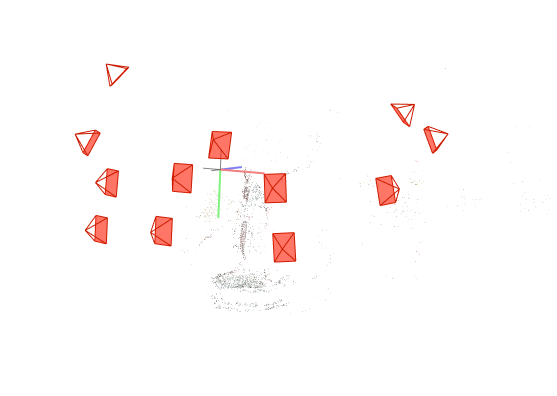
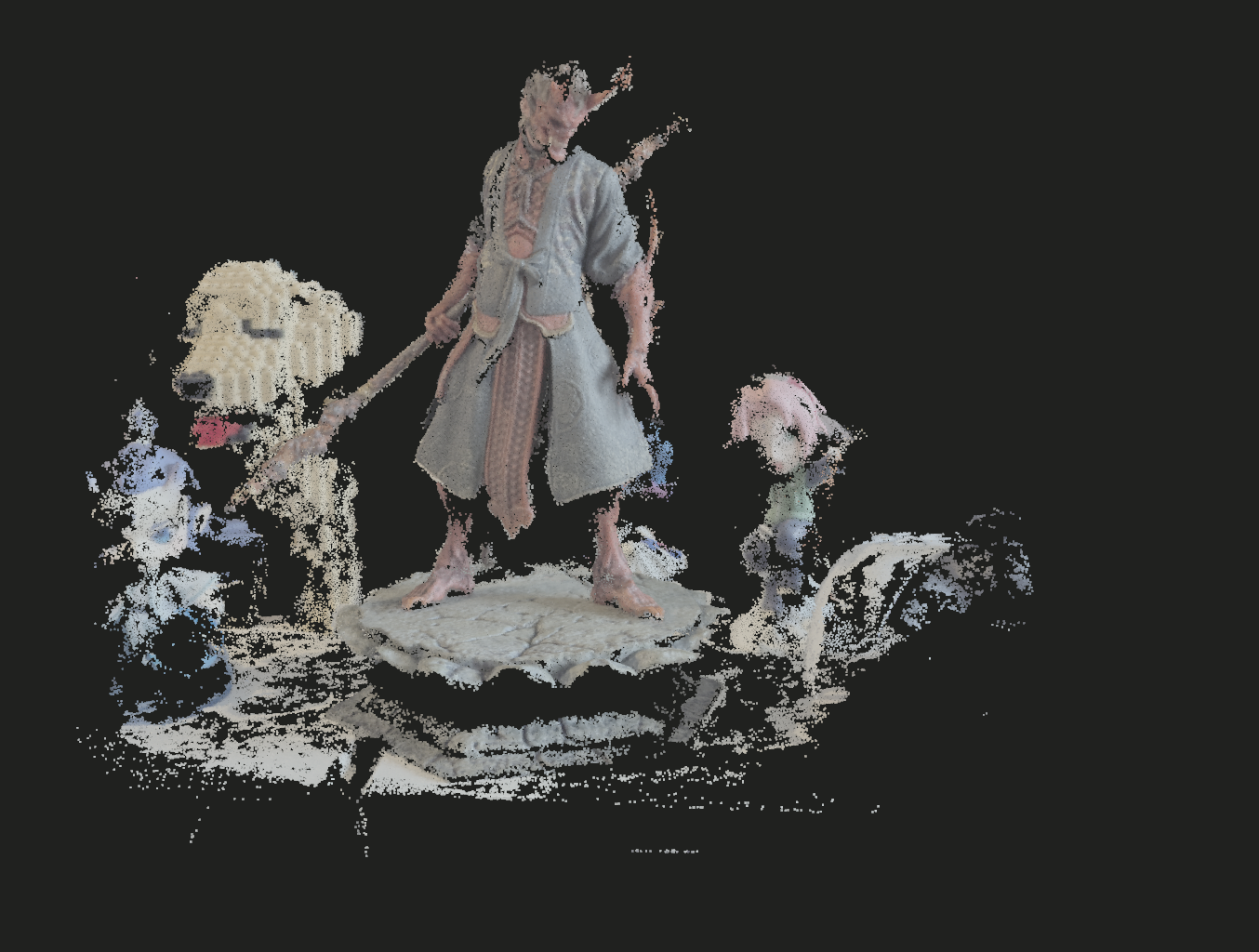
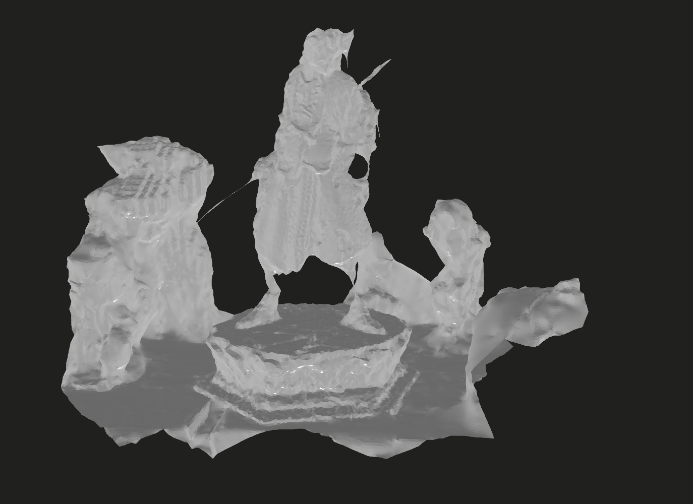
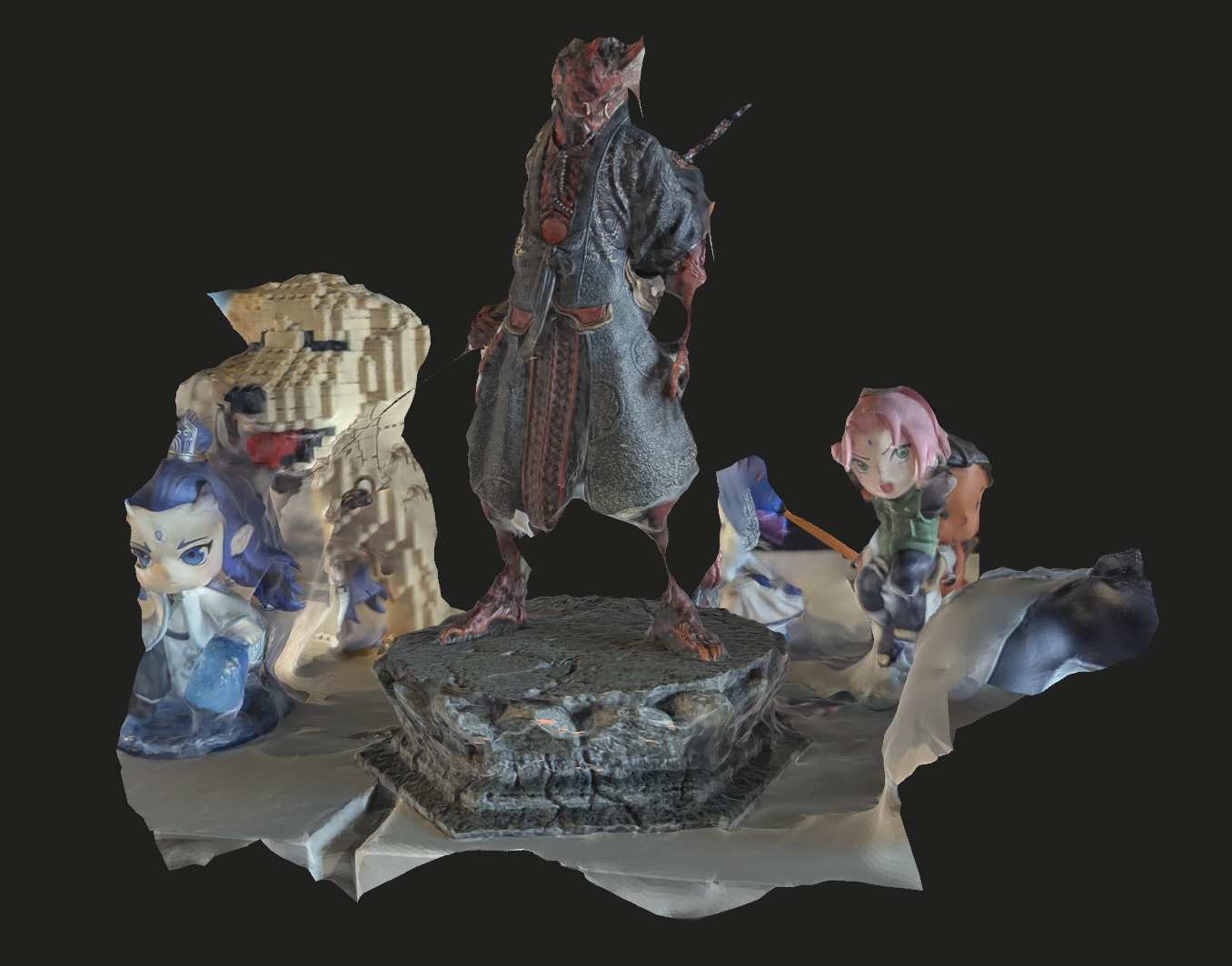
Example of sparse point cloud, dense point cloud, mesh and final textured obj
Multi-View Stereo
For a pixel $p_i=(u,v)$ in a reference image $I_i$, MVS estimates its depth $d=D_i(u,v)$ that makes the corresponding 3D point photometrically and geometrically consistent with other images.
Given camera $i$’s intrinsics $K_i$ and its pose $T_i\in SE(3)$, a world point $X$ observed by camera $i$ projects to
$$
p_i = \pi\left(K_iT_iX\right), \qquad \pi\left([x,y,z]^\top\right) = \left(x/z,,y/z\right),
$$
with $\pi(\cdot)$ the perspective projection (dehomogenization) that divides by depth.
Given a depth hypothesis $d$ for pixel $p_i$ in the reference view, the corresponding world point is recovered by following equation
$$
X(d) = T_i^{-1}\left(dK_i^{-1}\tilde{p}_i\right)
$$
where $\tilde p_i = (u,v,1)^T$ is the homogeneous coordinates
$X(d)$ is then re-projected into a neighboring image $I_j$:
$$
p_j(d) = \pi\left(K_jT_jX(d)\right).
$$
If $d$ is correct, the image patches around $p_i$ and $p_j(d)$ should look similar. This is measured with a matching cost $\rho$ (e.g., sum of squared differences or normalized cross-correlation over a patch window $\mathcal{W}$) between the two patches, aggregated over a set of neighboring source views $\mathcal{N}(i)$:
$$
C(p_i,d) = \sum_{j\in\mathcal{N}(i)} \rho\Big(I_i(\mathcal{W}(p_i)),, I_j(\mathcal{W}(p_j(d)))\Big).
$$
The estimated depth at $p_i$ is the hypothesis that minimizes this aggregated cost:
$$
\hat d(p_i) = \arg\min_{d} , C(p_i,d).
$$
Repeat the above steps for each pixel in each reference frame (suitable for GPU) could recovers the full depth map for each frame.
Usages of spare map in MVS
The camera intrinsics and poses are essential inputs to MVS. The sparse landmarks are not the final dense reconstruction, but they provide useful geometric guidance as depth prior for MVS.
- View Selection: images that observe many of the same sparse landmarks probably overlap. This information helps MVS choose source images that have both sufficient overlap and a useful baseline relative to the reference image.
- Depth-Range Initialization: The depths of nearby sparse landmarks can constrain the likely range.
TSDF and Mesh
Each depth map is expressed from the viewpoint of its reference camera. A valid depth pixel can be converted into a world-space point, so one possible intermediate result is a dense point cloud.
However, explicitly constructing a global dense point cloud is optional. The depth maps can be integrated directly into a volumetric representation such as a Truncated Signed Distance Function (TSDF):
During integration, each depth observation updates voxels near the measured surface. Observations from different views are combined using confidence or sensor-dependent weights. Repeated measurements reduce noise, while inconsistent or low-confidence measurements can be rejected or given less influence.
After fusion, a surface extraction algorithm such as Marching Cubes converts the zero level set of the TSDF into a triangle mesh.
Organizing the Voxels
A truncated SDF is only nonzero near the surface, so a dense 3D array covering the whole scene wastes most of its memory on empty space. Two spatial structures are commonly used instead:
- Voxel hashing stores voxels in fixed-size blocks, and hashes each occupied block’s 3D coordinate to a slot in a hash table. Only blocks near an observed surface are ever allocated, so memory scales with surface area rather than volume.
- Octrees recursively subdivide space into eight children, refining only where geometry is present, so resolution can also vary by region (e.g., finer near detailed surfaces, coarser elsewhere).
Neural Reconstruction
As the development of neural network, the submodule or the whole pipeline of reconstruction could be replaced with neural network approaches
Geometry Foundation model
Parts of the reconstruction modules like dense depth estimation could leverage neural network to solve, while there is also foundation model like VGGT that could replace the whole pipeline with end-to-end model approach.
$$
\text{Images}
\rightarrow \text{SfM/SLAM}
\rightarrow \text{MVS depth maps}
\rightarrow \text{TSDF fusion}
\rightarrow \text{mesh}.
$$
Feature extraction → matching → RANSAC → SfM → BA → MVS
Images → Transformer → Geometry
See more in the literature review post.
Implicit Scene Representations
Above approaches estimates the 3D geometry explicitly, either with classic or neural approach. An alternative family of methods instead optimizes a differentiable scene representation so that it reproduces the input images, and only implicitly encodes geometry as a byproduct.
A Neural Radiance Field (NeRF) represents a scene as a continuous function, typically an MLP, mapping a 3D point and viewing direction to a color and a volume density:
$$
F_\theta(x,d) \rightarrow (c,\sigma).
$$
To render a pixel, a ray $r$ is cast through the scene and sampled at points $x_1,\ldots,x_K$ along it. The pixel color is accumulated with the volume rendering integral:
$$
C(r) = \sum_{i=1}^{K} T_i\left(1-e^{-\sigma_i\delta_i}\right)c_i,
\qquad
T_i = e^{-\sum_{j<i}\sigma_j\delta_j},
$$
where $\delta_i$ is the distance between adjacent samples and $T_i$ is the accumulated transmittance up to sample $i$. Training minimizes the photometric error between $C(r)$ and the observed pixel color, over rays from all training images.
NeRF still depends on the earlier stages of the pipeline: it requires known camera intrinsics and poses for every training image, almost always obtained from SfM (e.g., COLMAP), exactly like MVS does.
What it changes is everything downstream of that: instead of estimating a depth map per view and fusing it, NeRF fits one global implicit volume per scene by test-time optimization, and geometry is recovered only indirectly through $\sigma$. A mesh can be extracted by running Marching Cubes on a level set of $\sigma$, but this is a secondary use — NeRF is optimized for photometric consistency, not surface accuracy, so extracted meshes are often noisier than MVS + TSDF results.
3D Gaussian Splatting (3DGS) keeps the same goal, optimizing a scene representation against posed input images, but replaces the implicit MLP with an explicit set of 3D Gaussian primitives. Each Gaussian $g_k$ has a position $\mu_k$, an anisotropic covariance $\Sigma_k$, an opacity $\alpha_k$, and a view-dependent color (typically spherical harmonics coefficients).
Rendering projects the 3D Gaussians onto the image plane and alpha-composites the resulting 2D splats, sorted by depth, instead of ray-marching a network:
$$
C(u,v) = \sum_{k} c_k,\alpha_k \prod_{k’<k}\left(1-\alpha_{k’}\right).
$$
Because splatting is a direct rasterization rather than a per-pixel network evaluation, 3DGS trains faster than NeRF and renders in real time, while still being optimized end-to-end from posed images with a photometric loss.
Initialization typically reuses the sparse point cloud from SfM to seed the initial Gaussian positions, so 3DGS also plugs into the pipeline right after the SfM/SLAM stage.
Compare with MVS + TSDF
| MVS + TSDF | NeRF | 3DGS | |
|---|---|---|---|
| Representation | Explicit depth maps $\to$ TSDF $\to$ mesh | Implicit radiance field (MLP) | Explicit set of 3D Gaussians |
| Optimized for | Multi-view photo-consistent depth | Photometric reconstruction of training views | Photometric reconstruction of training views |
| Fitting | Per-view depth estimation + fusion | Per-scene test-time optimization | Per-scene test-time optimization |
| Rendering new views | Not the primary goal | Ray marching (slow) | Rasterization (real time) |
| Geometry output | Mesh, metrically accurate by design | Density field; mesh extraction is secondary and noisier | Gaussian centers/point cloud; mesh extraction needs extra processing |
Both NeRF and 3DGS still rely on SfM or SLAM for camera poses, so they extend rather than replace the front half of the classic pipeline discussed above.
Open-Source Implementations
Famous implementations includes -
- OpenMVG (“Multiple View Geometry”): focuses on the SfM stage only.
- COLMAP: implements both SfM and MVS. Its SfM output format is the de facto standard input for NeRF and 3DGS training pipelines, while its dense reconstruction requires CUDA support.
- OpenMVS (“Multi-View Stereo”) : performs dense point-cloud estimation, mesh reconstruction, mesh refinement, and texturing on either CPU or GPU.