Manipulator Robotics Introduction

Posted on 2023-02-17 Edited on 2023-04-02 In Robotics

Notes of book Introduction ot Robotics Mechanics and Control.

Content

Focus on mechanical manipulator type of robot.

Table of content

Introduction
Describe pose in 3D
- Position & rotation
- Attach a coordinate system or frame to an object, then describe its pose w.r.t other reference coordinate systems
Geometry of mechanical manipulators. Static Kinematics
- Manipulator
  - consist of rigid links, which are connected by joints
  - joint angles (rotation), joint offset (translation)
  - tool frame is attached to end-effector
  - base frame is attached t o nonmoving base of manipulator
- Kinematics
  - Treats motions without regard to the forces which cause it
  - Study time-based properties of the motion
- Forward kinematics of manipulator
  - Given a set of joint angles, compute the pose of tool frame w.r.t the base frame
- Inverse kinematics of manipulator
  - Given the pose of end-effector of the manipulator, calculate all possible sets of joint angles
  - non-linear optimization problem
Kinematics with velocities and static forces
- Jocobian of manipulator
  - mapping from velocities in joint space to Cartesian space
- singularity of the mechanism
  - mechanism become locally degenerate and behaves as if it only has 1 DoF
Manipulator dynamics
- Study forces required to cause motion
Motion of manipulator. Trajectory in space
- Trajectory generation
  - spline: refer to a smooth function and passes through a set of via points
Mechanical design
- How to design a manipulator, including its mechanical structure, attached sensors
linear/non-linear control theory
- actuator perform torque on the joint
- position and velocity sensors are monitored by control algorithm
- linear control
  - linear approximations to the dynamics of a manipulator
- non-linear control
  - consider nonlinear dynamics
Active fore control
- Force control vs position control
Programming robots
Off-line simulation

Notation

$A$: vector or matrix
$a$: scalars
$^A P$: position vector under coordinate system {A}
$^A_B R$: rotation matrix {B} relative to {A}. $$^A P = ^A_B R ^B P $$
Vectors are taken to be column vectors

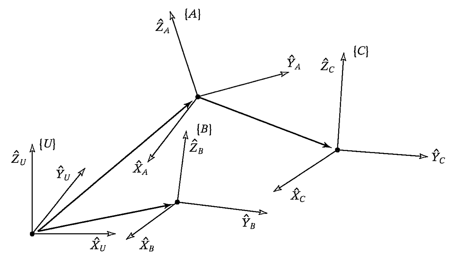
Spatial Descriptions and transformations

Position under universal coordinate frame {A}. $^A P$
- $^A P_{BORG}$ is the vector from frame {A} to frame {B} origin, and expressed under frame {A}
Rotation matrix (3x3), frame {B} relative to frame {A}
$$
^A_B R = [^A \hat{X}_B, ^A \hat{Y}_B, ^A \hat{Z}_B]
$$
where $^A \hat{X}_B, ^A \hat{Y}_B, ^A \hat{Z}_B$ are the coordinate of unit axes vectors of frame {B} in frame {A}. Row vectors are the axes vectors of frame {A} in frame {B} since $^B_A R = ^A_B R^{-1} = ^A_B R^T$

Maps position from frame {B} to frame {A}
$$
^A P = {^A_B R} {^B P} + ^A P_{BORG}
$$
or in homogenous coordinate, write as $^A_B T$
Transformation operators. Not transforming the frame, move the point under the same frame instead
$$
^A P_2 = T {^A P_1}
$$
The transform that rotates by $R$ and translate by $Q$ is the same as the transform that describes a frame rotated by $R$ and translated by $Q$ relative to the reference frame.
Other rotation forms
- 3 rotations taken about fixed axes （fixed-angle sets) yield the same final orientation as the same three rotations taken in opposite order about the axes of the moving frame (Euler-angle sets).
- Equivalent angle-axis representation $R_K(\theta)$. Rotating around unit vector $^A \hat{K}$ by $\theta$
- Euler parameters. Unit quaternion
Different vectors
- line vector: dependent on its line (or point) of action to cause its effect
- free vector: only its direction and magnitude matters, can be placed in anywhere in space
Reduce computation
- Compare matrix calculations vs matrix vector calculations
- Calculate first 2 columns, use cross product to get the third column

Manipulator Kinematics

Joints, Links

joint axis: revolute or prismatic
- joint 1 is the first movable joint in the robot
- joint n is the last movable joint in the robot
link: the arm. link $i$ is from axis $i$ to axis $i+1$
- link 0 is from the non-moving base of the robot to the first movable joint
- link n is from the last movable joint to the end-effector

Fixed Parameters
Changeable Parameters

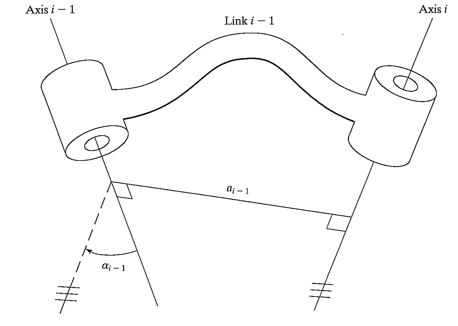
link length: length of line which is perpendicular to the 2 axes (mutual perpendicular, current axe and next axe)
- $a_i$ = distance from $\hat{Z}_i$ to $\hat{Z}_{i+1}$ measured along $\hat{X}_i$
- $a_0 = 0$ because axis joint $0$ could be chosen arbitrary
- $a_n = 0$ because there is no more other joints behind
link twist: angle in the projected plane from axis $i$ to axis $i+1$. The plane’s normal vector is $a_i$, the angle follows the right-hand law
- $\alpha_i$ = angle from $\hat{Z}_i$ to $\hat{Z}_{i+1}$ measured about $\hat{X}_i$
- $\alpha_0 = 0$ because axis joint $0$ could be chosen arbitrary
- $\alpha_n = 0$ becaus there is no more other joints behind

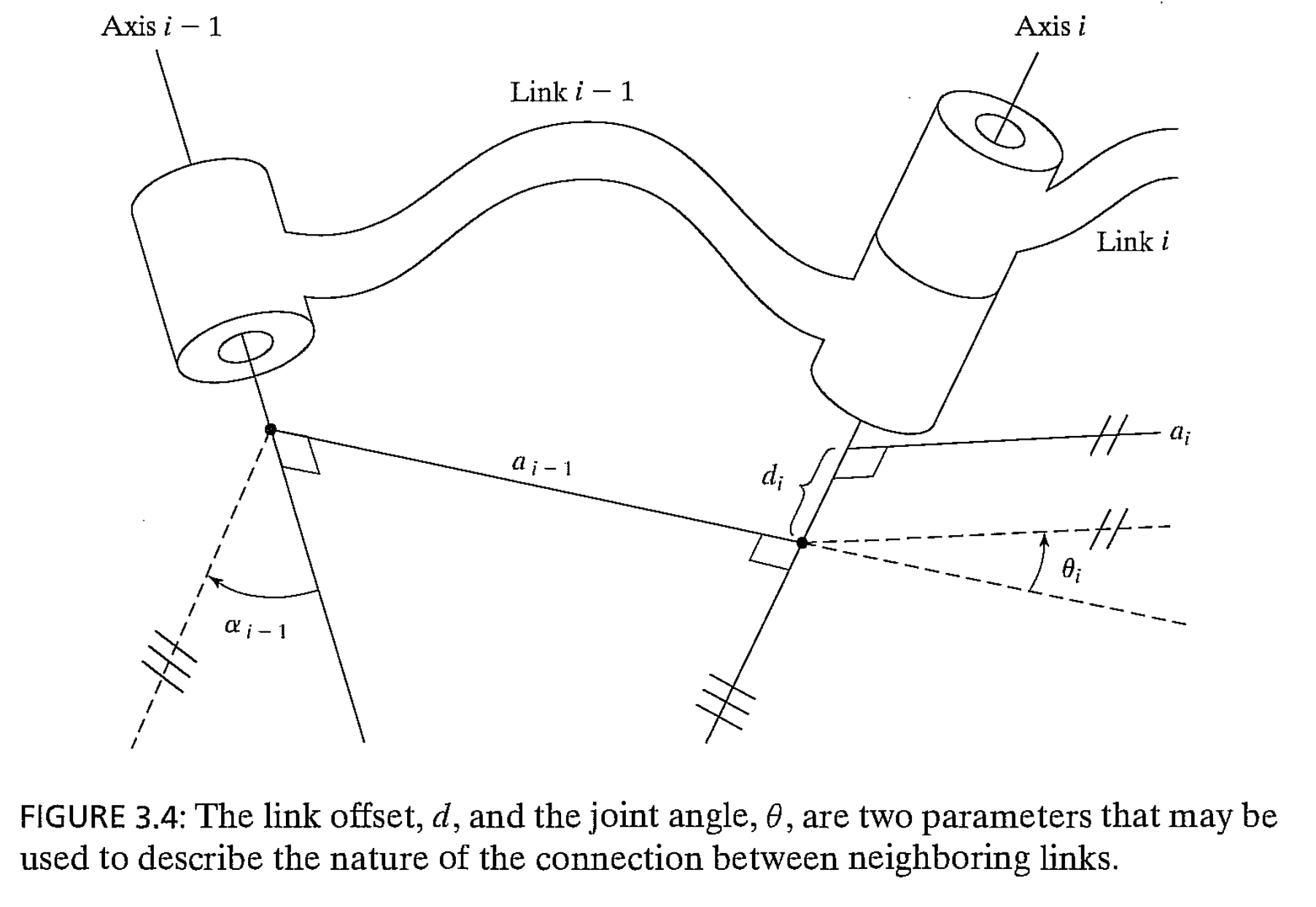
link offset: distance between intersection of $a_{i-1}$ on axis $i$ and $a_i$ on $i$. Distance is measured along the axis $i$
- $d_i$ = distance from $\hat{X}_{i-1}$ to $\hat{X}_i$ measured along $\hat{Z}_i$
- $d_1$
  - $d_1 = 0$ for revolute joint
  - $d_1$ zero position could be chosen arbitrary for prismatic joint
- $d_n$ same as above
joint angle: angle between from $a_{i-1}$ to $a_i$ around axis $i$. Also follows right-hand law
- $\theta_i$ = angle from $\hat{X}_{i-1}$ to $\hat{X}_i$ measured about $\hat{Z}_i$
- $\theta_1$
  - $\theta_1$ zero position could be chosen arbitrary for revolute joint
  - $\theta_1 = 0$ for prismatic joint
- $\theta_n$ same as above

link parameters: 3 fixed parameters
joint variable: 1 changeable parameter
- $\theta_i$ for revolute joint i
- $d_i$ for prismatic joint i

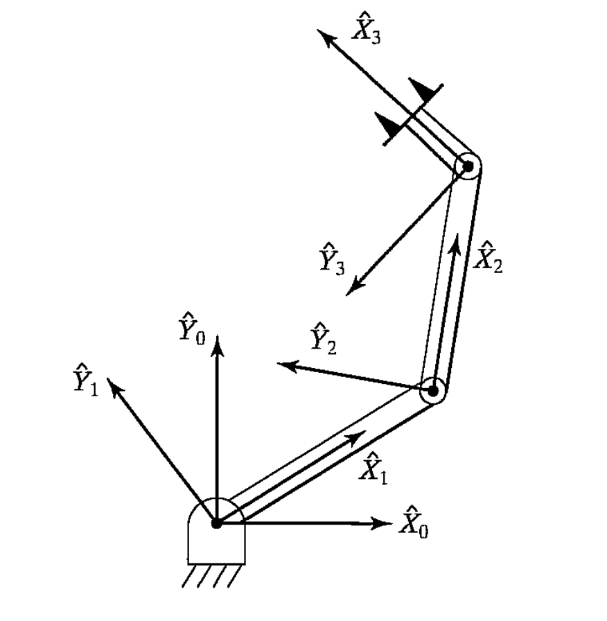
Frames

frame {i} attach to link i (axis i)
- Origin is the intersection point of the common perpendicular line on axis $i$.
- Z-axis coincident with joint axis i
- X-axis points along $a_i$ in the direction from joint $i$ to joint $i+1$
  - or orthonormal to the $Z_i, Z_{i+1}$ plane
- Frame {0} is arbitrary, but usually chose coincides with frame {1}. Frame {0} is the one stationary and serve as reference frame
- Frame {n}
  - X-axis is chosen it aligns with X-axis of frame {n-1} when $\theta_n = 0$
  - Origin is chosen at axis $n$ when $d_n = 0$

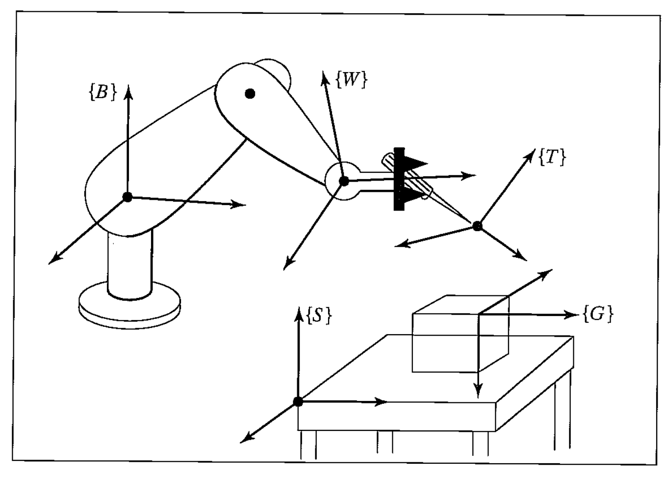
Frame naming convention
- Base frame {B}: frame {0}, link {0}, nonmoving
- Wrist frame {W}: frame {N}, last link the manipulator. Refer as $^B_W T = ^0_N T$
- Tool frame {T}: the end of any tool held by robot, or in the middle of fingertips. Refer as $^W_T T$
- Station frame {S}: task-relevant location, task frame, world frame, universal frame. Refer as $^B_S T$
- Goal frame {G}: location to which the robot is to move the tool. Tool frame and Goal frame will coincident in the end. Refer as $^S_G T$
WHERE function
- $^S_T T = ^B_S T^{-1} {^B_W T} {^W_T T}$, present where the tool is relative to the station

Frame kinematics transformation
$$
^{i-1}_i T=\begin{bmatrix}
\cos\theta_i & -\sin\theta_i & 0 & a_{i-1} \\
\sin\theta_i \cos\alpha_{i-1} & \cos\theta_i \cos\alpha_{i-1} & -\sin\alpha_{i-1} & -\sin\alpha_{i-1}d_i \\
\sin\theta_i \sin\alpha_{i-1} & \cos\theta_i \sin\alpha_{i-1} & \cos\alpha_{i-1} & \cos\alpha_{i-1} d_i \\
0 & 0 & 0 & 1
\end{bmatrix}
$$
$$
^0_N T = {^0_1 T} {^0_1 T} \cdots {^{N-1}_N T}
$$
$^0_N T$ is a function of $n$ joint parameters
Difference spaces
- actuator space: the parameters of actuators
- joint space: the space of the $n\times 1$ joint vector formed by $n$ joint variables
- Cartesian space: the relationship between different frames
Reduce computation
- Store sin cos values into lookup table
- Store intermediate variables

Inverse Manipulator Kinematics

What to solve: find the required joint angles to get the required $^S_T T$
- $^B_S T, ^W_T T$ are known
- Find required joint angles to get the required $^B_W T = ^0_N T$
Workspace: the volume of space that end-effector of manipulator can reach
- Dextrous workspace: volume of space that end-effector can reach with all orientations
- Reachable workspace: volume of space that end-effector can reach in at least one orientation
- But we usually care about the workspace of wrist frame {W} instead of the end-effector tool frame {T} since $^W_T T$ is known
- Workspace is a subset of the n-DoF subspace, where subspace is the reachable workspace without constraints of parameters
Solvable of inverse Kinematics
- Solution existence = desired position and orientation of wrist frame {W} is in the workspace
- Multiple solutions = desired position and orientation of wrist frame {W} is in the Dextrous workspace
  - 6 DoF manipulator could have up to 16 possible solutions
- Proved: all systems with revolute and prismatic joints having 6 DoF in a single series chain are solvable
  - But solution is in numerical
  - Closed-form solutions of 6 DoF is solvable in special cases
    - e.g. 3 neighboring joint axes intersect at a point
Method of solution
- numerical solutions: iterative method, slow, not guaranteed to find all solutions
- closed-form solutions
  - algebraic method
  - Geometric method
  construct the desired $^B_W T$ matrix (subspace) according to the required position and orientation
  
  construct equations between the constructed $^B_W T$ and kinematics matrix
  
  replace sin cos with single variable $u$, to convert transcendental equations to polynomial equations
  
  Proved. Polynomials up to degrees 4 could be solved in closed form
  forms triangles
Special cases
Pieper’s solution
- Any 3 DoF manipulator’s closed-from solution can be solved
- Compute a modified goal frame $^S_{G\prime} T$ such that $^S_{G\prime} T$ lies in manipulator’s subspace and is “near” to $^S_G T$
- Compute inverse kinematics for $^S_{G\prime} T$
Pieper’s solution to get closed-form solution
- Solve for first 3 joints given the position of the origin of frame {4} {5} {6}
- Solve for the later 3 joints given the orientation

Jocobians: velocities and static forces

Linear velocity vector for a point
$$
^A(^B V_Q) = {^A_B R} {^B V_Q} = \frac{^A d}{dt} {^B Q} = {^A_B R} \lim_{\Delta t \rightarrow 0} \frac{^B Q(t+\Delta t) - {^B Q(t)}}{\Delta t}
$$
is the velocity of position vector Q whose differentiation is done in frame {B} and finally expressed in frame {A}.
Short write cases
- $v_c = {^U V_{CORG}}$ is the velocity of origin of frame {C} differentiation in reference frame {U}
- $^A v_c$ is the above velocity but expressed in frame {A}

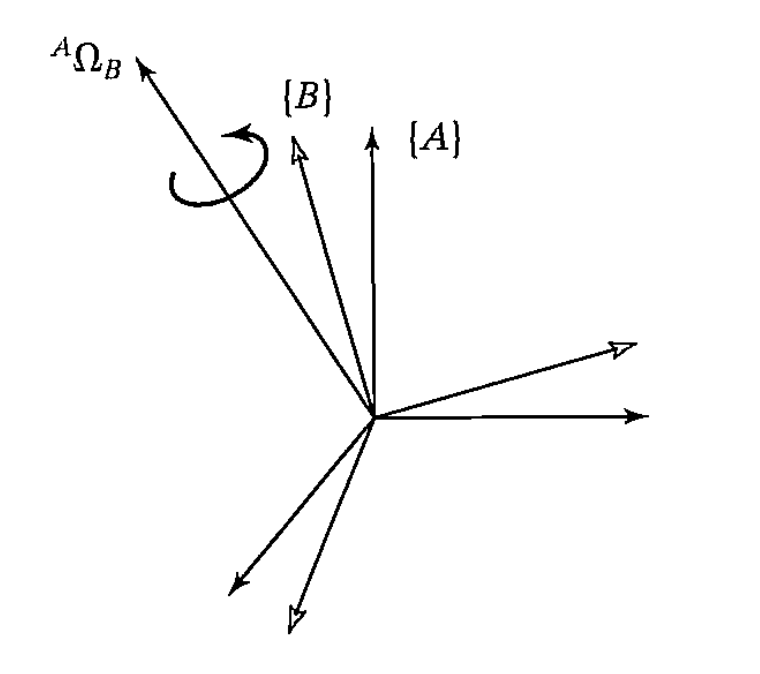
Angular velocity vector for a body
$$
^C ({^A \Omega_B})
$$
is the rotation of frame {B} relative to frame {A}, and finally expressed in frame {C}
- The direction of vector is the rotation axis
- The magnitude of vector is the current speed of rotation
Short write cases
- $w_c = {^U \Omega_C}$ is the angular velocity of frame {C} relative to reference frame {U}
- $^A w_c$ is the above angular velocity but expressed in frame {A}

Simultaneous linear and rotational velocity
$$
^A V_Q = {^A V_{BORG}} + {^A_B R} {^B V_Q} + {^A\Omega_B} \times {^A_B R} {^B Q}
$$
- where frame {A} is the reference frame and fixed
- frame {B} has both linear velocity $^A V_{BORG}$ and rotational velocity $^A \Omega_B$
- point Q also has a linear velocity $^B V_Q$ in frame {B}
Velocity of link i is given by vector $v_i$ and $w_i$, which are gotten relative to frame {0} and can be expressed in any frame
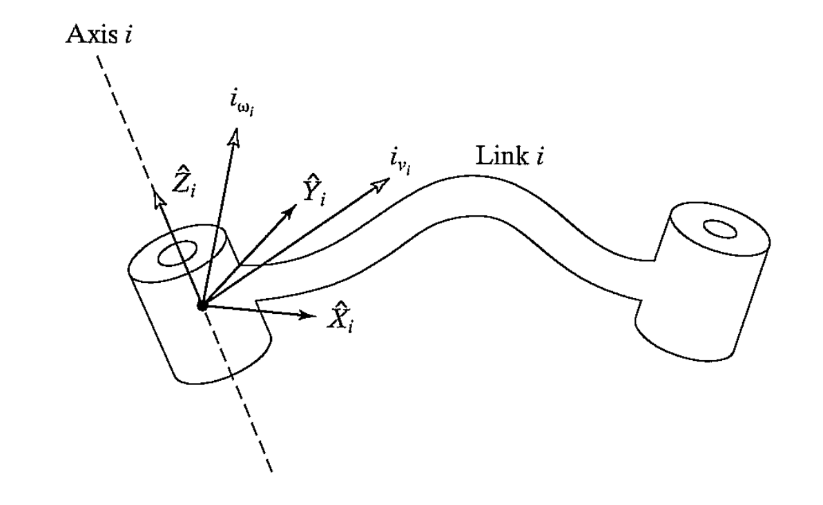
velocity propagation: velocity of link i+1 is velocity of link i, plus new velocity components added by joint i+1
- Revolute joint
- Prismatic joint
$$
\begin{aligned}
^{i+1} w_{i+1} &= {^{i+1}_i R} {^i w_i} + \dot{\theta}_{i+1} {^{i+1} \hat{Z}_{i+1}} \\
^{i+1} v_{i+1} &= {^{i+1}_i R} ({^i v_i} + {^i w_i} \times {^i P _{i+1}} )
\end{aligned}
$$

where
- $\dot{\theta}_{i+1} {^{i+1} \hat{Z}_{i+1}} = ^{i+1} \begin{bmatrix} 0 \\ 0 \\ \dot{\theta}_{i+1} \end{bmatrix}$
- $^i P_{i+1}$ is the coordinate of origin of frame {i+1} in frame {i}
$$
\begin{aligned}
^{i+1} w_{i+1} &= {^{i+1}_i R} {^i w_i} \\
^{i+1} v_{i+1} &= {^{i+1}_i R} ({^i v_i} + {^i w_i} \times {^i P _{i+1}} ) + \dot{d}_{i+1} {^{i+1} \hat{Z}_{i+1}}
\end{aligned}
$$

where $\dot{d}_{i+1} {^{i+1} \hat{Z}_{i+1}} = ^{i+1} \begin{bmatrix} 0 \\ 0 \\ \dot{d}_{i+1} \end{bmatrix}$
Velocity transformation
$$
\begin{aligned}
^A v_A &= {^A_B T_v} {^B v_B} \\
\begin{bmatrix}
^A v_A \\
^A w_A
\end{bmatrix}
&=
\begin{bmatrix}
^A_B R & {^A P_{BORG}} \times {^A_B R} \\
0 & {^A_B R}
\end{bmatrix}
\begin{bmatrix}
^B v_B \\
^B w_B
\end{bmatrix}
\end{aligned}
$$

Jocobian

Equation
$$
^0 v = {^0 J(\Theta)} \hat{\Theta}
$$
where
- $^0 v = \begin{bmatrix} {^0 v} \\ {^0 w} \end{bmatrix}$ is the Cartesian velocities of the link n expressed in frame {0}
- $\hat{\Theta}$ is the vector of joint velocity
- ${^0 J(\Theta)}$ is the Jocobian matrix, which represents the derivate of each term of Cartesian position and orientation on each term of joint angle. Its value changes as the joint angles change.
Changing frame
$$
{^A J(\Theta)} = \begin{bmatrix}
{^A_B R} & 0 \\
0 & {^A_B R}
\end{bmatrix}
{^B J(\Theta)}
$$
Inverse of the Jocobian could be used to calculate joint velocities given desired Cartesian velocities of link n
Singularities: where the joint angles make the ${^0 J(\Theta)}$ singular
- Workspace-boundary singularities: manipulator fully stretched out or folded back
- Workspace-interior singularities: caused by a lining up of 2 or more joint axes

Force and torque

Force propagation from link to link
$$
\begin{aligned}
^i f_i &= {^i_{i+1} R} {^{i+1}} f_{i+1} \\
^i n_i &= {^i_{i+1} R} {^{i+1}} n_{i+1} + {^i P_{i+1}} \times {^i f_i}
\end{aligned}
$$
where
- $f_i$ is force exerted on link i by link i-1
- $n_i$ is torque exerted on link i by link i-1
Torque for joint
- For revolute joint
  $$
  \tau_i = {^i n_i^T} {^i\hat{Z}_i}
  $$
- For prismatic joint
  $$
  \tau_i = {^i f_i^T} {^i\hat{Z}_i}
  $$
Jocobian
$$
\tau = {^0 J^T} {^0 \mathcal{F}}
$$
where $\mathcal{F}$ is the Cartesian forces acting at the hand, and $\tau$ is the joint torques
Force transformation
$$
\begin{aligned}
^A \mathcal{F}_A &= {^A_B T_f} {^B \mathcal{F}_B} \\
\begin{bmatrix}
^A F_A \\
^A N_A
\end{bmatrix}
&=
\begin{bmatrix}
^A_B R & 0 \\
{^A P_{BORG}} \times {^A_B R} & {^A_B R}
\end{bmatrix}
\begin{bmatrix}
^B F_B \\
^B N_B
\end{bmatrix}
\end{aligned}
$$
and
$$
{^A_B T_f} = {^A_B T_v^T}
$$

Trajectory generation

Motions is tool frame {T} relative to station frame {S}
To generate a trajectory of motions
- Spatial constraints: Path points
  - a set of intermediate frames that the tool frame should reaches
  - including initial, target point, and via points
- Temporal attributes: the time between points
In order to make the trajectory smooth, the function of the trajectory and its first derivate should be continuous

Joint-space schema
Cartesian-space schema

Convert path joints to joint angles by inverse kinematics
For each 2 path points, fit a function of the joint angles
Cubic polynomial
- 4 entries since each 2 path points provides 4 constraints (2 position constraints, 2 velocities constraints)
- $\theta(t) = a_0 + a_1 t + a_2 t^2 + a_3 t^3$
- Constraints of each 2 point
  $$
  \begin{aligned}
  \theta(t_0) &= theta_0 \\
  \theta(t_1) &= theta_1 \\
  \dot{\theta}(t_0) &= v_0 \\
  \dot{\theta}(t_1) &= v_1
  \end{aligned}
  $$
- Higher-order polynomials
  - Quintic polynomial (5 degree, 6 entires), enabling specify position, velocity, and acceleration.
- Linear function with parabolic blends

Reference

Rodd, Michael G. “Introduction to robotics: Mechanics and control: John J. Craig.” (1987): 263-264.