General Mathematic Basis for SLAM
This post talks about the fundamental math for SLAM, including Homogeneous Coordinates, Transformation in 3D space, Probability, SVD, Least Square Optimization, Lie Group and Lie Algebra and etc.
Homogeneous Coordinate
- Convert from Euclidean coordinate to Homogeneous coordinate
- For point: append an extra dimension with value 1
- For vector (point at infinity): append an extra dimension with value 0
- Convert from Homogeneous coordinate to Euclidean coordinate
- For point: divide other dimensions by the last dimensions and then drop the last dimension
- For vector (point at infinity): drop the last dimension
For point
$$
\begin{bmatrix}
1 \\
2 \\
3
\end{bmatrix} \rightarrow
\begin{bmatrix}
1 \\
2 \\
3 \\
1
\end{bmatrix} =
\begin{bmatrix}
2 \\
3 \\
6 \\
2
\end{bmatrix}
$$
For lines and planes, use the vector formed by coefficient of the line / plane equation to represent. e.g. line $3x + 4y + 5z + 6 = 0$ represented by $[3, 4, 5, 6]^T$.
More properties
- One coordinate multiplied by a non-zero scalar still represents the same point, e.g. $[2, 4, 1]^T = [4, 8, 2]^T$. This is also the definition of homogeneous coordinate
- Square sum of all dimensions cannot equal to 0. This is also the definition
- Setting last dimension to 0 could represent the point in infinitely far away, e.g. $[2, 4, 0]^T$. Even the point is far away, the direction information is still represented
- Setting dimensions except the last dimension to 0 could represent the line / plane in infinitely far away (horizon line), e.g. $[0, 0, 1]$ for line, $[0, 0, 0, 1]$ for plane.
- Dot production of 0 between line/plane and point coordinate means the point is inside the line/plane. $l \cdot x = l^T x = 0$
- Cross proudction between 2 lines or 2 planes could get the intersections $x = l_1 \times l_2$; Cross production between 2 points could get the line between the two points $l = x_1 \times x_2$
Coordinate Transformation: 3D Pose Representation
In 3D space, every object could be represented by a reference frame attached to it. There are 2 main reference frames.
- World reference frame $O_w$. Stationary. Usually chosen as the initial camera reference frame
- Camera reference frame $O_c$. Attached to camera, moving with camera.
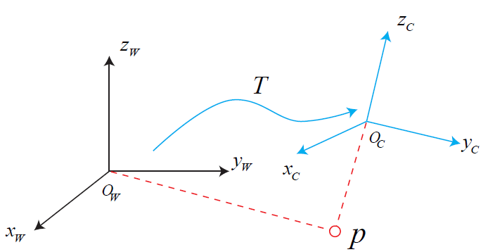
Then we can describe the camera pose inside the world reference frame using coordinate values under world reference frame.
- 3DoF Position: $t_{wc} \in \mathbb{R}^3$, the vector from world origin to camera origin, and is under world reference frame
- 3DoF Orientation: $R_{wc} \in \mathbb{R}^{3\times3}$, rotation matrix, columns are camera frame’s $x$, $y$, $z$ axle under world reference frame
- or quaternion $\mathbb{R}^4$, or euler angles $\mathbb{R}^3$, or axis-angle $\mathbb{R}^4$
Transformation matrix
By combing the position and orientation, we could get
$$
\begin{aligned}
\mathrm{SE(3)} &= \left\lbrace
T = \begin{bmatrix}
R & t \\
0^T & 1
\end{bmatrix}
\in \mathbb{R}^{4\times4} |
R \in \mathrm{SO(3)}, t \in \mathbb{R}^3
\right\rbrace \\
\mathrm{SO(3)} &= \lbrace R \in \mathbb{R}^{3\times3}|RR^T = I, \det( R )=1 \rbrace
\end{aligned}
$$
Specifically, we have
$$
T_{wc} = \begin{bmatrix}
R_{wc} & t_{wc} \\
0^T & 1
\end{bmatrix}
$$
The transformation matrix $T_{wc}$ could express different physical meanings as following.
$T_{wc}$ represents to transform the homogeneous coordinate of points / vectors from camera reference frame $O_c$ to world reference $O_w$.
For a space point $p$, there is
$$
\mathbf{p}_w = T_{wc} \mathbf{p}_c =
\begin{bmatrix}
\ R_{wc}p_c + t_{wc} \\
1
\end{bmatrix}$$
where
- $p_c$: coordinate of point p in camera reference frame $O_c$
- $\mathbf{p}_c$: homogeneous coordinate of point p in camera reference frame $O_c$
- $\mathbf{p}_w$: homogeneous coordinate of point p in world reference frame $O_w$
- $T_{wc}$: transformation of world frame from camera frame
- $R_{wc}$: column vectors are the coordinate of camera’s axe in world frame
- $t_{wc}$: vector from world origin to camera origin, and expressed under world frame
Note. $\mathbf{p}_c$ and $\mathbf{p}_w$ are different because the reference frame they expressed change, while the physical position of $p$ doesn’t change.
For a vector $v$, there is
$$
\mathbf{v}_w = T_{wc} \mathbf{v}_c =
\begin{bmatrix}
\ R_{wc}v_c \\
0
\end{bmatrix}$$
The difference is the homogeneous coordinate for a vector is to append $0$ in the end
$t_{wc}$
- Coordinate of camera origin in world frame $O_w$
- Vector from world origin to camera origin and under world frame $O_w$
$$
\mathbf{p}_w = T_{wc} \begin{bmatrix} 0 \\ 0 \\ 0 \\ 1 \end{bmatrix} = \begin{bmatrix}
\ t_{wc} \\
1
\end{bmatrix}
$$
$R_{wc}$
- Columns are camera’s axes in world frame $O_w$
- Rows are world’s axes in camera frame $O_c$
$$
\mathbf{v}_w^{(1)} = T_{wc} \begin{bmatrix}
1 \\
0 \\
0 \\
0 \\
\end{bmatrix}
=
\begin{bmatrix}
R_{wc}^{(2)} \\
0
\end{bmatrix},
\mathbf{v}_w^{(2)} = T_{wc} \begin{bmatrix}
0 \\
1 \\
0 \\
0 \\
\end{bmatrix}
=
\begin{bmatrix}
R_{wc}^{(2)} \\
0
\end{bmatrix},
\mathbf{v}_w^{(3)} = T_{wc} \begin{bmatrix}
0 \\
0 \\
1 \\
0 \\
\end{bmatrix}
=
\begin{bmatrix}
R_{wc}^{(3)} \\
0
\end{bmatrix}
$$
$T_{wc}$ could represent as a transformation operator to “move” the camera frame from world frame origin to where the camera frame is.
The columns of $R_{wc}$ could be constructed by angle $\theta_{cw}$, which is to rotate the reference frame from world frame origin to camera frame.
Also the $t_{wc}$ can also represent to translate the camera frame from the world origin’s position to camera origin’s position
Note. This is to operate the reference frame itself, it has the “reversed” meaning from transforming the coordinate of point between reference frames, where the reference frames are not moved.
$T_{wc}$ and $T_{cw}$
Since the transformation between reference frame is bi-directional. $T_{cw}$ could also be used to describe camera pose.
- $T_{cw} = T_{wc}^{-1}$: the coordinate transformation of camera frame $O_c$ from world frame $O_w$
- $R_{cw} = R_{wc}^{-1}$: column vector is the coordinate of world axes in camera frame
- $t_{cw} = -R_{wc}^{-1}t_{wc}$: vector from camera origin to world origin, and expressed under camera frame
The camera pose $T_{wc}$ or $T_{cw}$ is also called extrinsic, and it could also be transferred to a $\mathbb{R}^6$ vector using Lie Algebra.
Since both $T_{wc}$ and $T_{cw}$ could represent camera pose, we usually use the expressions of coordinate transformations and avoid to use the ambiguity term “camera pose”.
- The transformation of world frame from camera frame ($T_{wc}$)
- The transformation of camera frame from world frame ($T_{cw}$)
RANSAC (Random Sample Consensus)
- A method to eliminating the outlier data (seperate data into inliners and outliers). Steps are
- Sample the number of data required to fit the model
- Compute model using the sampled data points
- Score the model by the fraction of inliers within a preset threshold of the model
- Repeat the above steps until the best model is found
- Repeat Times $T$ of RANSAC to find the best model
$$
T = \frac{\log(1-p)}{\log(1-w^n)}
$$
where $p$ is the desired probability to find the best model, $w$ is the fraction of number of inliner to the number of whole data, and $n$ is the number of fit the model. - Properties
- The large $p$ or $n$, the more times required to perform RANSAC
- The large $w$, the less times required to perform RANSAC
- Good for model required little data points to fit
4 Fundamental Subspaces
For a matrix $A \in \mathbb{R}^{m\times n}$ with $rank(A) = r$, reduced to its row echelon form $R$ with LU factorization, there are four fundamental subspaces.
| Subspace | Dimension | Lives in | How to read it off |
|---|---|---|---|
| Row space $C(A^T)$ | $r$ | $\mathbb{R}^n$ | the pivot rows of $R$ |
| Null space $N(A)$ | $n - r$ | $\mathbb{R}^n$ | entries of $x$ corresponding to the non-pivot rows of $R$ |
| Column space $C(A)$ | $r$ | $\mathbb{R}^m$ | the columns of $A$ at the pivot positions of $R$ |
| Left null space $N(A^T)$ | $m - r$ | $\mathbb{R}^m$ | the last $m-r$ rows of $E$, where $EA = R$ |
The subspaces pair up as orthogonal complements:
- $C(A^T)$ and $N(A)$ are orthogonal complements in $\mathbb{R}^n$
- Any vector from one is orthogonal to any vector from the other, and together they span $\mathbb{R}^n$.
- A non-zero solution $x$ of $Ax=\mathbf{0}$ lies in $N(A)$, so it is orthogonal to every row of $A$.
- This doesn’t mean any vector from $\mathbb{R}^n$ is in either $C(A^T)$ and $N(A)$. Instead, any vector from $\mathbb{R}^n$ could be constructed by vectors from $C(A^T)$ and $N(A)$.
- $C(A)$ and $N(A^T)$ are orthogonal complements in $\mathbb{R}^m$ in the same way.
$A^TA$ is invertible when $A$ has full column rank
$A^TA$ shares the same null space as $A$. If $A$ has full column rank then $N(A) = \{\mathbf{0}\}$, so $A^TAx = \mathbf{0}$ has only the zero solution and $A^TA$ is invertible. This is what makes the least-square normal equations solvable.
Linear Equations
Set matrix $A \in \mathbb{R}^{m\times n}$, where $rank(A) = \min(m, n)$, vector $x \in \mathbb{R}^n$, vector $b \in \mathbb{R}^m$.
Matrix multiplication $Ax$ can be viewed as a linear combination of the columns of $A$, weighted by the entries of $x$.
Linear homogeneous equations
$$Ax = 0$$
$x = \mathbf{0}$ is always a solution, so the question is whether non-zero solutions exist. They form the null space $N(A)$, whose dimension $n - r$ depends only on the rank:
| Shape | Non-zero solutions of $Ax = \mathbf{0}$ |
|---|---|
| square or tall ($m > n$) with full column rank $r = n$ | none — only $x = \mathbf{0}$ |
| square or tall ($m > n$) with with rank ($r < n$) | infinitely many, spanning $N(A)$ of dimension $n - r$ |
| wide ($m < n$) | always infinitely many, since $r \le m < n$ |
To solve the equation:
$$
A x = \mathbf{0} \quad \begin{cases}
\begin{aligned}
m > n, \quad &\text{convert to least square problem} \\
&x^\star = \arg\min\limits_x ||Ax|| \ s.t. \ ||x|| = 1
\end{aligned} \\
\begin{aligned}
m < n, \quad &\text{use Gaussian elimination / LU factorization} \\
&x = \sum_{i=0}^{n-m} \lambda_i \xi_i
\end{aligned} \\
m = n = r, \quad \text{only have solution}, \quad x = 0
\end{cases}
$$
Solutions to solve least square problem of overdetermined equations.
Method 1: EVD of $A^TA$
$x^\star$ is the eigen vector respective to the least eigen value of $A^TA$
Proof
Convert optimization problem with constraints to non-constraints
$$
\begin{aligned}
&\min_x ||Ax|| \ s.t. \ ||x|| = 1 \\
\Rightarrow& \min_x (x^TA^TAx + \lambda (1-x^Tx))
\end{aligned}
$$
Compute the derivative of target function on $x$
$$
\frac{\mathrm{d} (x^TA^TAx + \lambda (1-x^Tx))}{\mathrm{d} x} = 2A^TAx - 2\lambda x \in \mathbf{R}^n
$$
The result $x^*$ is to make the derivative equals to 0, thus
$$
A^TAx^* = \lambda x^\star
$$
which means $x^\star$ is the eigen vector of $A^TA$, $\lambda$ is the eigen value of $A^TA$.
Bring back to the optimization problem
$$
\begin{aligned}
&\min_x (x^TA^TAx + \lambda (1-x^Tx)) \\
\Rightarrow& \min_x (x^T \lambda x) = \lambda
\end{aligned}
$$
Therefore, the minimal of optimization target is the least eigen value of matrix $A^TA$, and $x^\star$ is the respective eigen vector.
Method 2: SVD of $A$
$x^\star$ is the last column of matrix $V$, which is the SVD of $A=U\Sigma V^T$. See SVD section for more details
Linear non-homogeneous equations
$$Ax = b$$
A solution exists only when $\mathbf{b}$ lies in the column space $C(A)$, so the count depends on the rank as well as the shape:
| Shape | Solutions of $Ax = \mathbf{b}$ | Explanation |
|---|---|---|
| invertible square ($m = n = r$) |
exactly one | ~ |
| full-rank tall ($m > n = r$) |
at most one | The taller of the matrix, the harder its column to span the whole $R^m$ |
| full-rank wide ($m = r < n$) |
infinitely many | The wider of the matrix, the easier its column to span the whole $R^m$ |
| rank deficient ($r < m, r < n$) |
none, or infinitely many | Depending if there is a zero row equals to non-equal entry of $b$ |
Specifically for the full track scenario
- Full row rank means at least 1 solution
- since every row has its pivot. The condition of zero row equaling to non-zero entry of $b$ cannot happen
- the solutions depends on the number $n-r$
- Full column rank means at most 1 solution
- since every column has its pivot and there is no free column ($N(A)$ is ${0}$)
To solve the equations:
$$
A x = \mathbf{b} \quad \begin{cases}
\begin{aligned}
m < n, \quad &\text{use Gaussian elimination} \\
&x^\star = x_0 + \sum_{i=0}^{n-m} \lambda_i \xi_i
\end{aligned} \\
m = n, \quad x^\star = A^{-1}b \\
\begin{aligned}
m > n, \quad &\text{convert to least square problem} \\
&x^\star = \arg\min_x ||Ax - \mathbf{b}||
\end{aligned}
\end{cases}
$$
Note. If $rank(A|b) < rank(A)$, there is no solution, but could still convert to least square problem to get a approximated result.
Solutions to solve least square problem of overdetermined equations.
Method 1: Inverse of $A^TA$
$x^\star = (A^T A)^{-1}A^T\mathbf{b}$
Proof
Since
$$
||Ax - \mathbf{b}|| = x^TA^TAx - 2\mathbf{b}^T Ax + \mathbf{b}^T \mathbf{b}
$$
Then
$$
\frac{\mathrm{d} ||Ax - \mathbf{b}||}{\mathrm{d} x} = 2A^TAx - 2A^T \mathbf{b} \in \mathbb{R}^{n}
$$
To get the $x^\star$ which makes optimization target reaches minimal, we set its derivative to $\mathbf{0}$. (This cannot be the $x$ making optimization target reaches maximum value because the maximum value is infinity)
$$
x^\star = (A^TA)^{-1} A^T \mathbf{b}
$$
If applying SVD for matrix $A$, we could get
$$
x^\star = (V \Sigma^T U U \Sigma V^T)^{-1} V \Sigma^T U^T \mathbf{b} = V \Sigma^{-1} U^T \mathbf{b}
$$
Method 2: SVD of $A$
See SVD section for more details.
Projection
The projection of a vector $\mathbf{b}$ onto the line through $\mathbf{a}$ is the point on the line closest to $\mathbf{b}$:
$$
\mathbf{p} = \mathbf{a}\frac{\mathbf{a}^T\mathbf{b}}{\mathbf{a}^T\mathbf{a}}
$$
The projection of $\mathbf{b}$ onto a subspace $S$ is the vector $\mathbf{p} \in S$ such that the error $\mathbf{e} = \mathbf{b} - \mathbf{p}$ is orthogonal to $S$. When $S = C(A)$ and $A$ has full column rank,
$$
\mathbf{p} = A(A^TA)^{-1}A^T\mathbf{b} = P\mathbf{b}
$$
$P = A(A^TA)^{-1}A^T$ is the projection matrix.
When linear non-homogeneous equation $Ax = \mathbf{b}$ has no solution, we look for the $\hat{x}$ that
$$
\hat{x} = \arg\min_x || \mathbf{b} - Ax ||^2
$$
i.e. makes $Ax$ same the projection of $\mathbf{b}$ onto $C(A)$. This is the solution of the normal equations
$$
A^TAx = A^T\mathbf{b} \quad\Rightarrow\quad x = (A^TA)^{-1}A^T\mathbf{b}
$$
(the same result derived in Linear non-homogeneous equations). Numerically it is better solved through the QR decomposition below than by forming $A^TA$ directly.
Matrix Factorization
LU
Lower-upper Factorization is to use Gaussian elimination on matrix $A \in \mathbb{R}^{m\times n}$, to achieve a lower triangular matrix $L \in \mathbb{R}^{m \times m}$ and upper triangular matrix $U \in \mathbb{R}^{m \times n}$
$$
A = LU = \begin{bmatrix}
1 & 0 & \cdots & 0 \\
\star & 1 & \cdots & 0 \\
\vdots & \vdots & \ddots & \vdots \\
\star & \star & \cdots & 1
\end{bmatrix}
\begin{bmatrix}
\star & \star & \cdots & \star \\
0 & \star & \cdots & \star \\
\vdots & \vdots & \ddots & \vdots \\
0 & 0 & \cdots & \star
\end{bmatrix}
$$
$L$ has 1 in its diagonal and $U$ has pivots in its diagonal.
During the factorization, a sequence of lower-triangular elimination matrices turns $A$ into the upper-triangular $U$, i.e. $E_n \cdots E_2 E_1 A = U$. And we have
$$EA = U \rightarrow A = LU$$
Therefore, $L$ is the inverse of that sequence
$$
L = (E_n \cdots E_2 E_1)^{-1} = E_1^{-1} E_2^{-1} \cdots E_n^{-1}
$$
which is still lower triangular, each entry being the multiplier between rows used during elimination.
Variants:
- If a row swap is needed during elimination (since the row may not have pivot), a permutation matrix $P$ is applied (multiple swaps combine into one $P$, with $P^{-1} = P^T$), giving $PA = LU$.
- Pulling the pivots out of $U$ into a diagonal matrix $D$ gives $A = LDU$.
- For a symmetric $A$, this becomes $A = LDL^T$ where $D$ is the diagonal of pivots.
- Eliminating the entries above each pivot and normalizing the pivots to $1$ turns $U$ into the reduced row echelon form $R$.
Usages
converting to
$$
\begin{cases}
Ly = \mathbf{b} \\
Ux = y
\end{cases}
$$
Although the LU decomposition still requires Gaussian elimination, this is very helpful if the $\mathbf{b}$ keep changing.
Extension: LUP decomposition for non-square matrix, $P_{n\times m}A_{m\times n} = LU$
converting to
$$
\begin{cases}
Ly = P\mathbf{b} \\
Ux = y
\end{cases}
$$
Cholesky
A special LU decomposition for real symmetric positive definite matrix $A_{n\times n} = A^T$, where L is lower triangle matrix
$$
A = L L^T
$$
Usages
solve $Ax = \mathbf{b}$
converting to
$$
\begin{cases}
Ly = \mathbf{b} \\
L^T x = y
\end{cases}
$$
QR
QR Decomposition for matrix $A_{m \times n}$, and $m \geq n$, to a orthogonal matrix $Q$ and a upper triangle matrix $R$.
$$
A = Q_{m \times m} \begin{bmatrix}
R_{n \times n} \\
0_{(m - n) \times n}
\end{bmatrix}
$$
Use Gram-Schmidt to convert matrix $A = [a_1, \cdots, a_n]$ to orthogonal vectors $[q_1, \cdots, q_n] = A T$, where matrix $T$ is an upper triangle matrix, and its inverse is matrix $R$, which is still an upper triangle matrix.
Usages
$$A_{m\times n} = Q_{m\times n}R_{n\times n} \rightarrow Q^TAQ = RQ$$
Let $A_2 = RQ$, whose eigenvectors are same with $A$. Repeat the QR decomposition, until the $A_n$ is a diagonal matrix.
$$
\begin{split}
x^\star &= (A^T A)^{-1}A^T\mathbf{b} = (R^TQ^TQR)^{-1}R^TQ^T\mathbf{b} \\
&=(R^TR)^{-1}R^TQ^T\mathbf{b} \\
&=R^{-1}Q^T\mathbf{b}
\end{split}
$$
EVD
Eigenvalue Decomposition for square matrix $A_{n\times n}$
$$
A V = V \Sigma
$$
where $V = [v_1, v_2, \cdots, v_n]$ and $v_i$ is the eigenvector, and $\Sigma = diag(\lambda_1, \lambda_2, \cdots, \lambda_n)$ is the eigenvalue. So
$$
A = V \Sigma V^{-1}
$$
Diagonalizable of the matrix
This is called the diagonalization of a matrix. Specifically,
- Whether $A$ has a zero eigenvalue decides whether $A$ is invertible.
- Whether $A$ has repeated eigenvalues decides whether $A$ is diagonalizable:
- Eigenvectors of distinct eigenvalues are always independent, so if all eigenvalues differ, $A$ is diagonalizable.
- For a repeated eigenvalue, the number of independent eigenvectors is at most its multiplicity; $A$ is diagonalizable only when there are enough independent eigenvectors.
- When diagonalizable, $A = X \Lambda X^{-1}$ using the (independent) eigenvector matrix $X$. This makes high powers $A^k = X \Lambda^k X^{-1}$, which is very trivial to compute.
Symmetric
A real symmetric matrix $S$ always has $n$ real eigenvalues (possibly repeated) and $n$ orthogonal eigenvectors, so its diagonalization turns to be
$$
S = Q \Lambda Q^{-1} = Q \Lambda Q^T
$$
Positive-definite matrices
For any matrix, the number of positive eigenvalues equals the number of positive pivots.
For a symmetric matrix $S$, it is positive definite when any of these equivalent conditions hold:
- all pivots are positive;
- all eigenvalues are positive;
- all leading principal determinants are positive;
- $x^T S x > 0$ for any $x \neq \mathbf{0}$;
- $S = A^T A$ for some $A$ whose columns are all independent.
Usages
$A \approx V_{n\times r} \Sigma_{r\times r} V_{n\times r}^{-1}$
converting to
$$
\begin{cases}
V y = b \\
\Sigma z = y \\
V^{-1} x = z
\end{cases}
$$
SVD
Singular Value Decomposition is a useful method to solve equations or estimate a matrix, so we put it into a separate section.
If we have a matrix $A$ with size $m\times n$, we could have its SVD like
$$
A = U \Sigma V^T
$$
where
| Element | Size | Meaning |
|---|---|---|
| $U$ | $m \times m$ | formed by eigenvectors of $A A^T$ |
| $\Sigma$ | $m \times n$ | diagonal matrix where values are singular value, $\sigma_i = \sqrt{\lambda_i}$, and $\lambda_i$ are the eigen values of $A A^T$ and $A^T A$ |
| $V$ | $n \times n$ | formed by eigenvectors of $A^T A$ |
A few notes:
- Since $A A^T$ and $A^T A$ are symmetric matrix, their eigen vectors are gurantted to be orthonormal. Therefore we have $U^T = U^{-1}$ and $V^T = V^{-1}$.
- The first $r$ columns of $U$ are a basis of $C(A)$, the last $m - r$ a basis of $N(A^T)$.
- The first $r$ columns of $V$ are a basis of $C(A^T)$, the last $n - r$ a basis of $N(A)$.
- Since $x^T A^T A x = || Ax ||^2 \geq 0$, the matrix $A$ is semi positive-definite, therefore their eigen values $\lambda_i \geq 0$
- The singular values $\sigma_1 \geq \sigma_2 \geq \cdots \geq \sigma_r > 0$ are the square roots of the non-zero eigenvalues of $A A^T$ and $A^T A$
Usages
$A \approx U_{m \times r} \Sigma_{r \times r} V_{r \times n}^T$
Target
$$
\min_x || Ax || \quad s.t. \quad || x || = 1
$$
where $A \in \mathbb{R}^{m\times n}$, and $m > n$, which means there are more observations than unknown
$$
\begin{split}
&\min_x || Ax || = \min_x || U\Sigma V^T x || \\
=& \min_x || \Sigma V^T x || \\
=& \min_y || \Sigma y || = \min_y y^T \Sigma^T \Sigma y \\
=& \min_y \Sigma_{i=0}^k y_i^2 \sigma_i^2 \quad s.t. \quad ||y|| = 1
\end{split}
$$
Explanation
If a matrix $B^T = B^{-1}$, then
$$
|| Bx || = x^T B^T B x = x^T x = || x ||
$$
For vector $y$, we also have $|| y || = 1$. The reason is because
$$
V^T x = \begin{bmatrix}
e_1^T \\
e_2^T
\end{bmatrix} x = \begin{bmatrix}
e_1^T x \\
e_2^T x
\end{bmatrix} = \begin{bmatrix}
\cos (\theta) \\
\cos (\frac{\pi}{2} - \theta)
\end{bmatrix}
$$
where $\theta$ is the angle between unit vector $e_1$ and $x$
Therefore, when the $y^* = [0, 0, \cdots, 1]^T$, then $\min || Ax || = \sigma_k^2$
Then $x^* = (V^T)^{-1} y^* = V [0, 0, \cdots, 1]^T$, which means $x^*$ is the last column of matrix $V$.
Target
$$
\min_x || Ax - \mathbf{b}||
$$
where $A \in \mathbb{R}^{m\times n}$, and $m > n$, which means there are more observations than unknown
$$
\begin{split}
&\min_x || Ax - \mathbf{b}|| = \min_x || U\Sigma V^T x - \mathbf{b} || \\
=& \min_x || \Sigma V^T x - U^T \mathbf{b} || \\
=& \min_y || \Sigma y - \mathbf{b}^{\prime} ||
\end{split}
$$
Then $y^\star = \Sigma^{-1} \mathbf{b}^\prime = [\frac{\mathbf{b}^{\prime}_0}{\sigma_0}, \cdots, \frac{\mathbf{b}^{\prime}_n}{\sigma_n}]^T = V^Tx^\star$
And $x^\star = Vy^\star = V\Sigma^{-1}\mathbf{b}^\prime = V \Sigma^{-1} U^Tb$
Physical meaning
Eigen vector has the property
$$
A v_i = \sigma_i u_i
$$
$v_i$ and $u_i$ represents the major direction for the subspace before and after the transformation of matrix $A$
The SVD can also be written as a sum of rank-1 terms
$$
A = \sigma_1 u_1 v_1^T + \cdots + \sigma_r u_r v_r^T
$$
therefore
- The closest lower-rank matrix to $A$ is obtained by setting the smallest singular values to $0$.
- $|| A || = \sigma_1$, the largest singular value, which is also the maximum of $|| Ax || / || x ||$.
Pseudo-inverse
The pseudo-inverse is $A^+ = V \Sigma^+ U^T$, where $\Sigma^+$ takes the reciprocal of each non-zero entry of $\Sigma$. Through $A v_i = \sigma_i u_i$ and $A^+ u_i = \frac{1}{\sigma_i} v_i$:
- $A$ maps the row space $C(A^T)$ to the column space $C(A)$, and the null space $N(A)$ to $\mathbf{0}$.
- $A^+$ maps the column space $C(A)$ back to the row space $C(A^T)$, and the left null space $N(A^T)$ to $\mathbf{0}$.
Eigenvalues and Eigenvectors
For a square matrix $A$, an eigenvector $x$ and eigenvalue $\lambda$ satisfy
$$
Ax = \lambda x
$$
Some properties
- The sum of the eigenvalues equals $trace(A)$; their product equals $det(A)$.
- $A^2$ has eigenvalues $\lambda^2$, $A^{-1}$ has $1/\lambda$, $A + I$ has $\lambda + 1$, and $A^T$ keeps the same $\lambda$.
- Similar matrices $B = P^-1 A P$ share the same eigenvalues.
- Repeatedly multiplying a vector by $A$ leaves the component along the eigenvector with the largest $|\lambda|$.
- Special matrices:
- Orthogonal matrix: $\lambda = \pm 1$ (since $Q^{-1} = Q^T$).
- Projection matrix: $\lambda \in \{0, 1\}$ (since $P^2 = P$).
- Reflection matrix: $\lambda = \pm 1$.
- Diagonal / triangular matrix: eigenvalues sit on the diagonal.
- Singular matrix ($det(A) = 0$): $0$ is an eigenvalue, because $Ax = \mathbf{0}$ has a non-zero solution.
Linear Transformation
A transformation $T$ is linear when $T(c\mathbf{v} + d\mathbf{w}) = cT(\mathbf{v}) + dT(\mathbf{w})$, which also forces $T(\mathbf{0}) = \mathbf{0}$.
Every linear transformation can be represented by a matrix $A$:
- It maps a vector of space $V \subseteq \mathbb{R}^n$ to space $W \subseteq \mathbb{R}^m$, so $A$ is $m \times n$.
- The matrix depends on the chosen bases of $V$ and $W$; different bases give different $A$ for the same transformation.
- Column $i$ of $A$ is $T(\mathbf{v}_i)$, the image of the $i$-th input basis vector expressed in $W$’s basis.
Identity transformation $T(\mathbf{v}) = \mathbf{v}$ is described by a square matrix: choosing the standard basis gives $A = I$; choosing input basis $V$ and output basis $W$ gives $B = W^{-1}V$.
Same input/output dimension (square $A$ under the standard basis):
- If $A$ has $n$ independent eigenvectors $B$ (i.e. is diagonalizable), choosing them as the input and output basis gives $B^{-1}AB = \Lambda$, the eigenvalue matrix.
- Otherwise, padding with extra vectors to form $B$ gives the Jordan form $B^{-1}AB = J$, where each padding vector puts a $1$ above its eigenvalue.
Different input/output dimension (standard-basis matrix $A$): choosing the input basis as $V$ (right singular vectors) and the output basis as $U$ (left singular vectors) gives $U^{-1}AV = \Sigma$, the diagonal singular-value matrix.
Derivative of Matrix (Jacobian Matrix)
$x = [x_1, \cdots, x_n]^T \in \mathbb{R}^n $
Scalar on Vector
$f(x) \in \mathbb{R}$
$$
\frac{\mathrm{d}f}{\mathrm{d}x} = \left[ \frac{\mathrm{d}f}{\mathrm{d}x_1}, \cdots, \frac{\mathrm{d}f}{\mathrm{d}x_n} \right]^T \in \mathbb{R}^n
$$
or
$$
\frac{\mathrm{d}f}{\mathrm{d}x^T} = \left[ \frac{\mathrm{d}f}{\mathrm{d}x_1}, \cdots, \frac{\mathrm{d}f}{\mathrm{d}x_m} \right] \in \mathbb{R}^{1 \times n}
$$
Specifically, if $b\in\mathbb{R}^n$
$$
\frac{\mathrm{d} (b^Tx)}{\mathrm{d} x} = b \in \mathbb{R}^n
$$
Vector on Vector
$F(x) = [f_1(x), \cdots, f_m(x)]^T \in \mathbb{R}^m$
$$
\frac{\partial F}{\partial x^T} = \begin{bmatrix}
\frac{\partial f_1}{\partial x^T} \\
\vdots \\
\frac{\partial f_m}{\partial x^T}
\end{bmatrix} = \begin{bmatrix}
\frac{\mathrm{d}f_1}{\mathrm{d}x_1} & \cdots & \frac{\mathrm{d}f_1}{\mathrm{d}x_n} \\
\vdots & \ddots & \vdots \\
\frac{\mathrm{d}f_m}{\mathrm{d}x_1} & \cdots & \frac{\mathrm{d}f_m}{\mathrm{d}x_n}
\end{bmatrix}
\in \mathbb{R}^{m \times n}
$$
Specifically, if $A\in\mathbb{R}^{m\times n}$
$$
\frac{\mathrm{d} (Ax)}{\mathrm{d} x^T} = A \in \mathbb{R}^{m\times n}
$$
Lie Group and Lie Algebra
- Group: $G = (A, \cdot)$
- Lie Group: continuous group
- Lie Algebra: $(V, F, [])$
$SO(3)$ and $so(3)$
$$
SO(3) = \lbrace R \in \mathbb{R}^{3\times3}|RR^T = I, det( R )=1 \rbrace
$$
For $R_1 \in SO(3)$ and $R_2 \in SO(3)$, $R_1 R_2 \in SO(3)$
Lie Algebra $so(3)$
$$
so(3) = \lbrace \phi \in \mathbb{R}^3, \Phi=\phi^{\wedge} \in \mathbb{R}^{3\times3} \rbrace
$$
For $\phi_1 \in so(3)$ and $\phi_2 \in so(3)$, $[\phi_1, \phi_2] = [ \Phi_1\Phi_2 - \Phi_2\Phi_1 ]^{\vee} \in so(3)$
Convert $SO(3) \Leftrightarrow so(3)$
For respective $R \in SO(3)$ and $\phi \in so(3)$
$$
\begin{split}
R &= \exp(\phi^{\wedge}) = \sum_{n=0}^{\infty}\frac{(\phi^{\wedge})^n}{n!} \\
&= \cos\theta I + (1 - \cos\theta) aa^T + \sin\theta a^{\wedge}
\end{split}
$$
where $\phi = \theta a$, a is a vector with $||a|| = 1$.
$$
\begin{aligned}
a^{\wedge}a^{\wedge} = aa^T - I \\
a^{\wedge}a^{\wedge}a^{\wedge} = -a^{\wedge}
\end{aligned}
$$
$$
\begin{split}
\phi &= \ln(R)^{\vee} = (\sum_{n=0}^{\infty} \frac{(-1)^n}{n+1} (R+I)^{n+1})^{\vee} \\
&= \theta a =
\begin{cases}
\theta = \arccos\frac{tr(R) - 1}{2} \\
\text{solve} \ a \ \text{by} \ Ra = a
\end{cases}
\end{split}
$$
$SE(3)$ and $se(3)$
$$
SE(3) = \left\lbrace T =
\begin{bmatrix}
R & t \\
0 & 1
\end{bmatrix}
\in \mathbb{R}^{4\times4}|R \in SO(3), t \in \mathbb{R}^{3}
\right\rbrace
$$
For $T_1 \in SE(3)$ and $T_2 \in SE(3)$, $T_1 T_2 \in SE(3)$
$$
se(3) = \left\lbrace \xi =
\begin{bmatrix}
\rho \\
\phi
\end{bmatrix} |
\rho \in \mathbb{R}^{3}, \phi \in SO(3)
\right\rbrace
$$
For $\xi_1 \in se(3)$ and $\xi_2 \in se(3)$, $[\xi_1, \xi_2] = [ \xi_1^{\wedge}\xi_2^{\wedge} - \xi_2^{\wedge}\xi_1^{\wedge} ]^{\vee} \in se(3)$
$$
\xi^{\wedge} =
\begin{bmatrix}
\phi^{\wedge} & \rho \\
0^T & 0
\end{bmatrix}
\in
\mathbb{R}^{4 \times 4}
$$
Convert $SE(3) \Leftrightarrow se(3)$
For respective $T \in SE(3)$ and $\xi \in se(3)$
$$
\begin{split}
T &= \exp(\xi^{\wedge}) = \sum_{n=0}^{\infty}\frac{(\xi^{\wedge})^n}{n!} \\
&= \begin{bmatrix}
\exp(\phi^{\wedge}) & J\rho \\
0^T & 1
\end{bmatrix}
\end{split}
$$
where
$$
J = \frac{\sin\theta}{\theta} I + \left( 1 - \frac{\sin\theta}{\theta} \right) aa^T + \frac{1 - \cos\theta}{\theta} a^{\wedge}, \ \phi = \theta a
$$
$$
\xi = \begin{bmatrix}
\rho \\
\phi
\end{bmatrix} =
\begin{cases}
\theta = \arccos\frac{tr(R) - 1}{2} \\
\text{solve} \ a \ \text{by} \ Ra = a \\
t = J\rho
\end{cases}
$$
Derivative of Lie Algebra
Derivative of $so(3)$
The derivative of $\frac{\partial Rp}{R}$ is hard to calculate because the $SO(3)$ have constraint and cannot do addition, where $R \in SO(3)$ is rotation matrix, $p \in \mathbb{R}^{3}$ is a point in space. But we can calculate the derivative of respective Lee Algebra $\phi$.
$$
\begin{split}
\frac{\partial \exp(\phi^{\wedge})p}{\partial \phi^T}
&= \lim_{\delta\phi \rightarrow 0} \frac{\exp((\delta\phi)^{\wedge})\exp(\phi^{\wedge})p - \exp(\phi^{\wedge})p}{\delta\phi^T} \\
&= \lim_{\delta\phi \rightarrow 0} \frac{(I + (\delta\phi)^{\wedge})\exp(\phi^{\wedge})p - \exp(\phi^{\wedge})p}{\delta\phi^T} \\
&= \lim_{\delta\phi \rightarrow 0} \frac{(\delta\phi)^{\wedge}\exp(\phi^{\wedge})p}{\delta\phi^T} \\
&= \lim_{\delta\phi \rightarrow 0} \frac{-(\exp(\phi^{\wedge})p)^{\wedge}\delta\phi}{\delta\phi^T} \\
&= -(\exp(\phi^{\wedge})p)^{\wedge} \\
&= -(Rp)^{\wedge} \in \mathbb{R}^{3\times 3}
\end{split}
$$
For the derivative on point $p$
$$
\begin{split}
\frac{\partial \exp(\phi^{\wedge})p}{\partial p^T} = p
\end{split}
$$
Derivative of $se(3)$
Similarily, the derivative to $T \in SE(3)$ can also be finished in Lee Algebra $\xi \in se(3)$, and point in homogeneous coordiante $\mathbf{p} = [x \ y \ z \ 1]^T = [p^T \ 1]^T$
$$
\begin{split}
\frac{\partial \exp(\xi^{\wedge})\mathbf{p}}{\partial \xi^T}
&= \lim_{\delta\xi \rightarrow 0} \frac{\exp((\delta\xi)^{\wedge})\exp(\xi^{\wedge})\mathbf{p} - \exp(\xi^{\wedge})\mathbf{p}}{\delta\xi^T} \\
&= \lim_{\delta\xi \rightarrow 0} \frac{(I + (\delta\xi)^{\wedge})\exp(\xi^{\wedge})\mathbf{p} - \exp(\xi^{\wedge})\mathbf{p}}{\delta\xi^T} \\
&= \lim_{\delta\xi \rightarrow 0} \frac{(\delta\xi)^{\wedge}\exp(\xi^{\wedge})\mathbf{p}}{\delta\xi^T} \\
&= \lim_{\delta\xi \rightarrow 0} \frac{\begin{bmatrix}
(\delta\phi)^{\wedge} & \delta\rho \\
0^T & 0
\end{bmatrix}
\begin{bmatrix}
Rp + t \\
1
\end{bmatrix}}{\delta\xi^T} \\
&= \lim_{\delta\xi \rightarrow 0} \frac{\begin{bmatrix}
(\delta\phi)^{\wedge}(Rp + t) + \delta\rho \\
0^T
\end{bmatrix}}{[\delta\rho^T \quad \delta\phi^T]} \\
&= \begin{bmatrix}
I_{33} & -(Rp+t)^{\wedge} \\
0^T & 0^T
\end{bmatrix} \in \mathbb{R}^{4\times 6}
\end{split}
$$
The result is a $4\times 6$ matrix, and the $R, t$ can be extracted from $T \in SE(3)$, which can be calculated from $\xi \in se(3)$ by $\exp(\xi^{\wedge})$.
If we drop the last row, we can get
$$
\frac{\partial (Rp + t)}{\partial \xi^T} = \begin{bmatrix}
I_{33} & -(Rp+t)^{\wedge}
\end{bmatrix}
$$
For the derivative on point $p$
$$
\frac{\partial \exp(\xi^{\wedge})\mathbf{p}}{\partial p^T} = \frac{\partial (Rp + t)}{\partial p^T} = R
$$
Probability Theory
- Probability
- Marginalization
- Indenpence / Conditional Indenpence
- Bayes Rules
$$ P(x|y) = \frac{P(y|x)P(x)}{P(y)} $$- Joint Probability $P(x|y)$
- Likelihood Probability $P(y|x)$, prior probability $P(x)$
- Background Knowledge $z$ besides $x, y$
$$
P(x|y, z) = \frac{P(y|x, z) P(x|z)}{P(y | z)}
$$
- Normal (Gauss) Distribution
- 1-d, N-d
- The multivariate normal distribution of k-dimensional random vector $\mathbf{X}=(X_1, \cdots, X_k)^T$, which is $$\mathbf{X} \sim \mathcal{N}(\mu, \Sigma)$$
The distribution is
$$
f_{\mathbf{X}}(x_1, \cdots, x_k) = \frac{1}{((2\pi)^k |\Sigma|)^{1/2}} \exp\left( -\frac{1}{2} (\mathbf{x}-\mu)^T \Sigma^{-1} (\mathbf{x}-\mu) \right)
$$
- The covariance matrix $\Sigma$ is symmetric and positive semi-definite, it could be diagonalizable as $\Sigma = Q \Lambda Q^T$.
Least square with covariance matrix
For $b = A\mathbf{x}$, the covariance propagates as $Cov(b) = A V A^T$.
When solving overdetermined $Ax = b$. If the components of $\mathbf{b}$ are independent, we have $x = (A^TA)^{-1}A^T\mathbf{b}$.
If they are correlated with covariance $V$, we got
$$
A^TV^{-1}Ax = A^TV^{-1}\mathbf{b} \Rightarrow x = (A^TV^{-1}A)^{-1}A^TV^{-1}\mathbf{b}
$$
The covariance of the estimate is
$$
Cov(x) = [(A^TV^{-1}A)^{-1}A^TV^{-1}] V [(A^TV^{-1}A)^{-1}A^TV^{-1}]^{-1} = (A^TV^{-1}A)^{-1}
$$
Special Matrices
- Square matrices:
- Identity: the neutral element.
- Diagonal: pivots and eigenvalues both sit on the diagonal.
- Symmetric: real eigenvalues and $n$ orthogonal eigenvectors; diagonalizable into an orthogonal matrix and an eigenvalue matrix.
- Orthogonal: easy to invert ($Q^{-1} = Q^T$), ideal for solving invertible linear systems.
- (upper/lower) Triangular: convenient for solving linear systems by substitution.
Six Great Theorems of Linear Algebra
- Dimension Theorem: All bases for a vector space have the same number of vectors.
- Counting Theorem: Dimension of column space + dimension of nullspace = number of columns.
$$ \dim(C(A)) + \dim(N(A)) = n $$ - Rank Theorem: Dimension of column space = dimension of row space. This common value is the rank.
- Fundamental Theorem: The row space and nullspace of $A$ are orthogonal complements in $\mathbb{R}^n$.
- SVD: There are orthonormal bases ($\mathbf{v}$’s and $\mathbf{u}$’s for the row and column spaces) so that $A\mathbf{v}_i = \sigma_i \mathbf{u}_i$.
- Spectral Theorem: If $A^T = A$ there are orthonormal $\mathbf{q}$’s so that $A\mathbf{q}_i = \lambda_i \mathbf{q}_i$ and $A = Q \Lambda Q^T$.