Survey of Visual Inertial SLAM
This post goes through the popular Visual Inertial SLAM systems, including MSCKF, OKVIS, VINS-Mono and etc.
Introduction
Visual inertial SLAM, or Visual inertial odometry (VIO), is an instance of SLAM. They used particular visual (usually monocular camera) and inertial sensors (gyroscope and accelerator).
For each system, following components will be covered.
- Sensor Type: IMU with monocular, stereo, and RGBD
- Frontend
- Initialization (mainly for monocular camera)
- Tracking
- Relocalization
- Loop Closure Detection
- Backend
- Mapping (map management)
Similar to other SLAM system, VIO can be categorized by feature-based or direct method frontend, filter or optimization-based backend, or VI-SLAM vs VIO based on whether it has the loop closure detection and build a global consistency map. In this post, we name both VI-SLAM and VIO as VIO.
Since VIO uses two types of sensor, a more obvious categorized method is the type of 2 sensors’ fusion.
Tightly-coupled vs Loosely-coupled Sensor Fusion
| ~ | Loosely-coupled | Tightly-coupled |
|---|---|---|
| Method | Process visual and inertial measurements separately to get the pose, then use them together | Directly fuse the visual and inertial measurements to get the pose |
| Forms | Usually is filter based | Could use filter method or batch estimation method |
| Pros | Computationally efficient | Higher accuracy |
Different from visual SLAM where batch estimation usually has higher accuracy, filter and batch estimation methods for visual inertial SLAM system behave very similarly. This is because the involvement of IMU data reduces the dependencies on the historical measurements to estimate the states.
MSCKF
A multi-state constraint Kalman filter for vision-aided inertial navigation
MSCKF_VIO, OpenVINS
Anastasios Mourikis, University of California
Highlights
- Proposed a deeply-coupled, sliding-window, filter-based visual inertial odometry framework with very low computation cost
- Derive the constraints for a 3D mappoint to be observed in multiple frames, and use it in the EKF step, which avoids to put 3D mappoint position in the EKF state, reducing the computation cost
- Computation cost is linear to the number of feature observations, up to cubic of sliding window
- Camera observations are grouped per 3D mappoint, instead of per camera
Drawbacks
- Not jointly update the mappoints’ position
- Don’t have relocalization and loop closure module
Architecture
- Sensor type: monocular camera and IMU
- Initialization: none
- Tracking and mapping are based on EKF (Extended Kalman Filter)
- Maintain a state vector of current IMU state and several camera pose, with their covariance matrix
- Prediction step
- Every time a new IMU measurement is received, the IMU term in the state vector will be updated using the Runge-Kutta numerical integration, and the covariance matrix will also be updated to reflect the correlation between IMU state and camera states
- Every time a new image is received, the state vector will be augmented by appending a new camera pose in the end, the camera pose is calculated by current IMU state and the previous calibration between camera and IMU
- Update step
- When a feature that has been tracked in a number of images is on longer detected, or old camera states will be removed from the sliding window because maximum number of camera frame reaches
- For each mappoint, its 3D position is calculated by triangulation from different camera and their observations
- For each mappoint, compute its residual, which is the multi-state constraint involving several camera’s error states from main EKF state
- For all mappoints’ residuals, perform QR decomposition and calculate the Kalman gain, and update the EKF state vector and covariance matrix
- No relocalization
- No loop closure detection
- Construct spare map
- Add new frame into EKF state for each new image
- Delete old frames from EKF state if the number of frames in EKF state exceeds the pre-defined threshold
- Add mappoints with valid position before using it for EKF update
- No obvious mappoint deletion because mappoint is not included in EKF update. But each mappoint will be used for EKF update once
EKF State
- Current IMU state. 16 parameters. 4 for rotation quaternion, 3 for translation, 3 for velocity, 3 for gyro bias, 3 for accelerator bias
- A sliding window of camera pose. For each pose
- rotation quaternion
- translation
The transformation matrix between camera and IMU is previous calibrated.
Mappoint Parameterization
The parameterization of 3D mappoint is inverse depth. It includes the following property for the first camera frame that observes this mappoint
- direction vector $[\alpha, \beta, 1]^T$
- inverse depth $\rho = \frac{1}{d}$
Using vector + “depth” is because the depth has larger uncertainty compared to the other 2 dimensions.
Using inverse depth instead of depth directly is because the inverse depth could has better linearization when calculate the 1st order Jocobian of the measurement (the 2nd derivative is much smaller compared to the 1st derivate). For more info, refer to the paper Unified Inverse Depth Parametrization for Monocular SLAM.
Analysis of EKF
MSCKF uses sliding window EKF, which contains several previous camera poses. When performing the EKF update, both latest IMU state and the previous camera states will be updated, thus though it is in filter form, it is batch estimation.
However, compared to the sliding window batch optimization like VINS-mono, MSCKF won’t optimize the mappoint position jointly with poses, leading it not optimal.
As for the EKF update step, the residual of each mappoint is only determined by the camera states instead of the IMU state, but there is correlation between IMU state and camera states in the covariance matrix. Therefore, during the EKF update step, both the IMU state and the camera states will be updated.
OKVIS
Keyframe-based Visual-Inertial SLAM using Nonlinear Optimization
Github
ETH Zurich
Highlights
- Proposed a deeply-coupled, sliding-window, optimization-based visual inertial odometry framework
- Sliding window maintenance uses keyframe concepts
Drawbacks
- Computation cost when performing data association
Architecture
- Sensor type: stereo cameras and IMU
- Initialization
- A bounded set of camera frames is maintained
- All landmarks visible in these images are kept in the local map
- Keypoints are stereo-triangulated
- All first $N$ frames are considered as keyframes
- Tracking
- Extract multi-scaled SSE-optimized Harris corner keypoints and compute BRISK descriptor in 2 stereo frames
- Descriptors are extracted oriented along the gravity direction (projected into the image)
- Keypoints are stereo-triangulated and inserted into a local map
- Perform brute-force keypoints matching against all of the map landmarks
- Outlier rejection is performed by applying a chi-square test in image coordinates by using the (uncertain) pose predictions obtained by IMU integration
- Add state and new landmarks into sliding window of frames, and remove old frames from this window to marginalization window
- This is the sliding window containing most recent $N$ frames
- Marginalize previous states if reaches the maximum window size
- This is the sliding window containing N keyframes. Frames moved from frames window will be put this window to perform marginalization
- Perform visual inertial optimization on the sliding window containing recent frames
- Extract multi-scaled SSE-optimized Harris corner keypoints and compute BRISK descriptor in 2 stereo frames
Sliding Window Optimization
- State vector (several frames and several mappoints)
- For each frame (15 DoF): pose (6-DoF), velocity (3-DoF), accelerator bias (3-DoF), gyro bias (3-DoF)
- For each landmark (3 DoF): position in homogeneous coordinate
- Optimization cost function
- Reprojection Error Formulation
- IMU Kinematics
- IMU Measurement Error Term
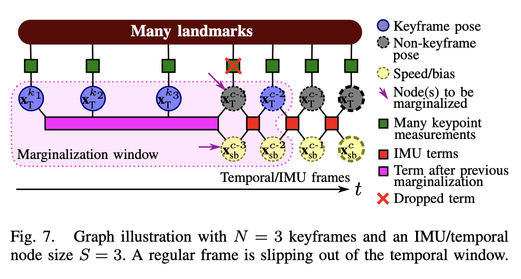
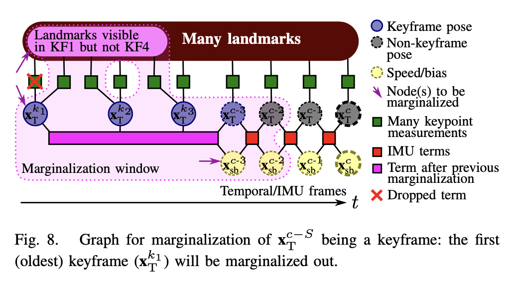
Sliding Window Marginalization
Determine keyframe by ratio between image area spanned by matched points vs area spanned by all detected points
When new frame $c$ is inserted into optimization window
- If oldest frame $c-S$ is not a keyframe, drops its keypoints observations, and marginalize its speed and bias state out
- If oldest frame $c-S$ is a keyframe, marginalize out the landmarks that are visible in first keyframe in marginalization window but not in most recent keyframe.
VINS-Mono
A Robust and Versatile Monocular Visual-Inertial State Estimator
Github
HKUST
Highlights
- Full Visual Inertial SLAM system with initialization, loop closure, global optimization, map reuse
- Robust initialization process
- Could handle both large scale tracking and realtime AR use cases
Drawbacks
- AR use case is not optimal as full mode
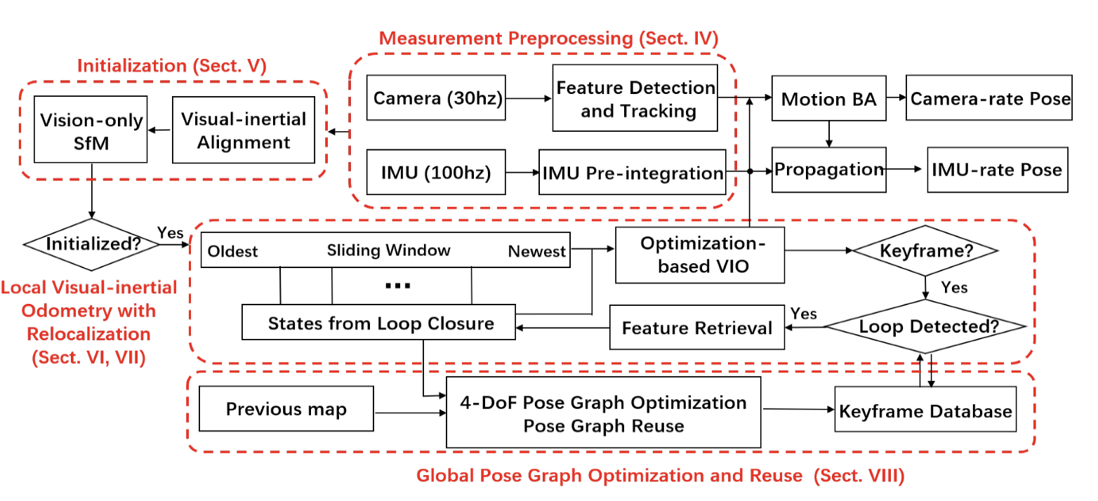
Architecture
- Sensor type: monocular camera and IMU
Initialization
- Vision-only SfM in Sliding Window
- Maintain a sliding window for several frames
- Extract new corner features for new frame, tracking existing feature with KLT sparse optical flow
- Select the previous frame which has enough feature matches with latest frame
- Perform 2D-2D 5-point algorithm to get the up to scale relative pose from reference frame and latest frame
- Triangulate 3D mappoints from these 2 frames
- Use 3D-2D PnP method to calculate other frames’ pose
- Bundle adjustment for the sliding window to optimize all feature measurements
- Set the first frame as reference frame, transform all frame pose under the first frame
- Visual-inertial Alignment
- IMU measurements are pre-integrated between every 2 frame
- Gyroscope bias calibration
- Linearize IMU measurements in terms of gyroscope bias, minimizing the cost function of relative rotation from vision-only SfM to solve the gyroscope bias for each frame
- Velocity, gravity vector and metric scale initialization
- Construct cost function with data from vision-only SfM to estimate velocities for each frame, gravity vector in first frame, and metric scale
- Accelerometer bias is not optimized in this process
- Gravity refinement
- Refine the gravity since the magnitude of gravity is assumed as known
- Completing initialization
- Compute the world frame whose z-axis is aligned with gravity direction, from the first camera frame and the gravity vector
- Rotate all poses and positions into the world frame
- Vision-only SfM in Sliding Window
- Tracking and mapping (based on sling window batch estimation)
- Extract new corner features for new frame, tracking existing feature with KLT sparse optical flow
- Determine whether the new frame is a keyframe according to the average parallax apart from the previous keyframe and the tracking quality
- Add frame state and observed features into sliding window
- Marginalize old states from the sliding window
- Based on whether the 2nd latest frame is keyframe
- Performs sliding window optimization
- If is keyframe, adds to PoseGraph
- PoseGraph only contains keyframes
- Each keyframe has its 6DoF pose, velocity, feature positions & descriptors
- Links between keyframe are 4DoF pose (3DoF position + yaw angle) since roll and pitch are observable due to IMU input, so they won’t drift
- Extract new corner features for new frame, tracking existing feature with KLT sparse optical flow
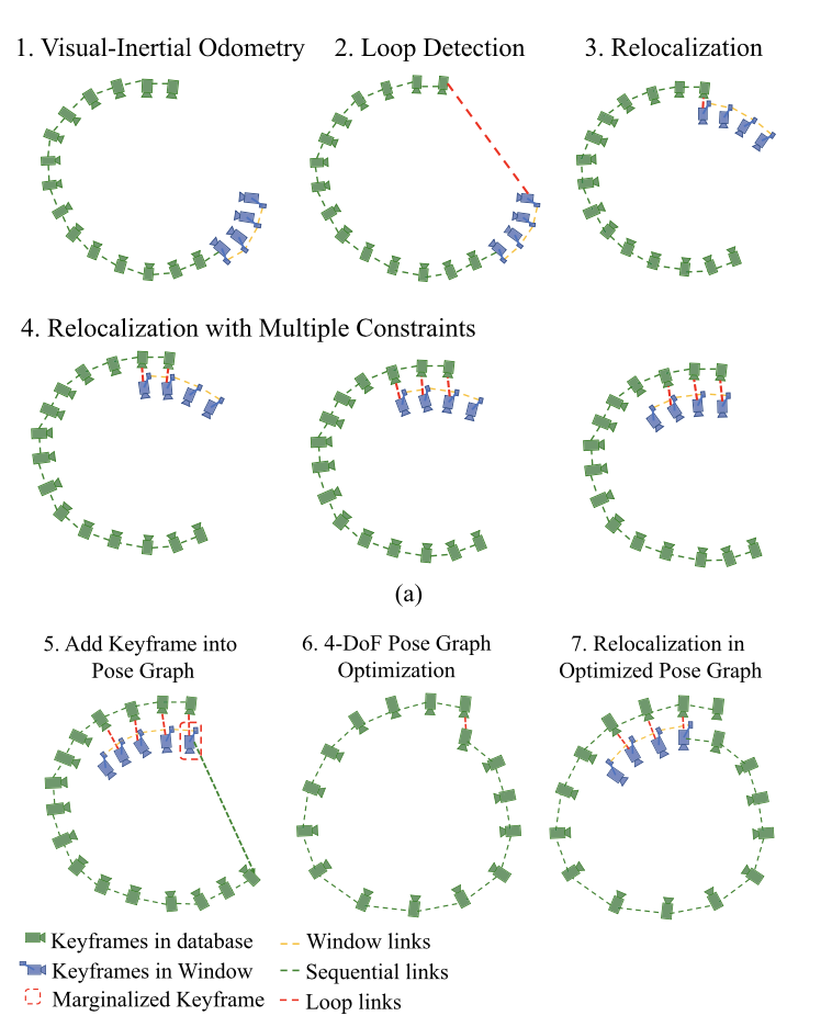
- Relocalization & loop closure
- Only process for new keyframe
- Detect 500 more corner features and compute BRIEF descriptors
- Use DBoW2 to perform loop closure detection with all detected descriptors
- BRIEF descriptor feature matching with outlier rejection
- 2D-2D: compute fundamental matrix with RANSAC
- 3D-2D: use previous mappoints in loop frame, compute PnP with RANSAC
- Optimize VIO window poses to align window frame to loop frame
- Keep loop frames fixed
- States: pose and landmarks inside sliding window
- Measurements:
- IMU measurements
- Visual measurements
- Feature correspondences between loop frames and new keyframe
- Also optimize loop frames
- Keep loop frames fixed
- Perform global pose graph optimization
- Global pose graph optimization & map reuse
- Construct and solve the pose graph optimization
- States: 4DoF pose (3DoF position + yaw angle) of each keyframe
- Measurements
- Existing relative keyframe link (4 DoF) when adding keyframes, without robust kernel
- Next detected loop closure pose link (4 DoF), with robust kernel
- Map reuse requires to detect loop closure between current active map and existing old map, then perform the global pose graph optimization
- Construct and solve the pose graph optimization
- Construct sparse map
Sliding Window
- States
- Several cameras’ states (15 DoF): pose (6-DoF), velocity (3-DoF), accelerometer bias (3-DoF), gyroscope bias (3-DoF)
- Several mappoints’ inverse depth
- The mappoint is reference from the first observing frame
- Extrinsic between IMU and camera (6-DoF)
- Measurements
- IMU pre-integration
- Feature measurements
- Using unit sphere camera model to deal with different camera type
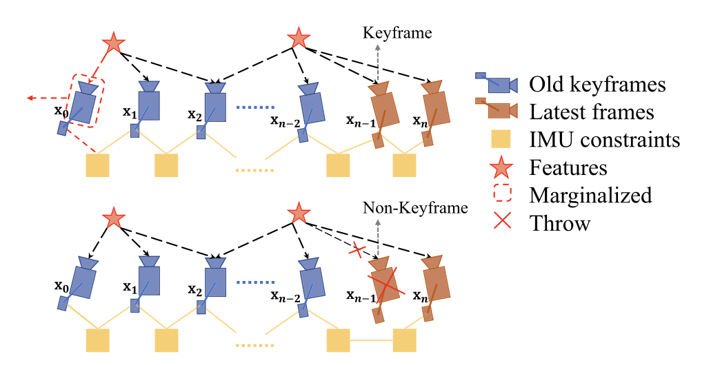
- Marginalization of previous frame and mappoints
- Window maintenance
- Add new frame and observing points to the window
- Marginalize frame when the window reaches the maximum
- If the 2nd latest frame is keyframe, marginalize the oldest frame and its observing mappoints
- If the 2nd latest frame is normal frame, just remove its state and observations, leave its pre-integration
- Keyframe is determined when extracting new features from the frame. Either of the following needs to meet
- Average parallax of features from previous keyframe is larger than threshold
- Tracking quality is poor
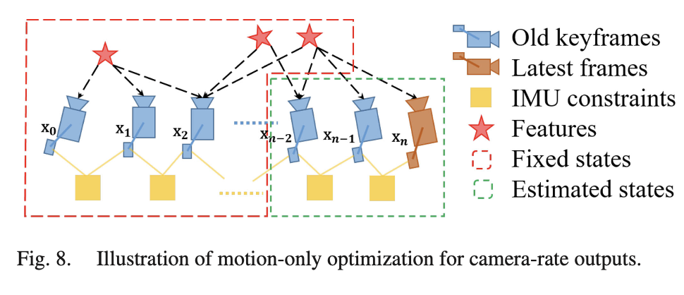
Different tracking modes
There is a tracking mode for mobile AR use cases. The steps are as following.
- Track existing feature with KLT sparse optical flow
- Maintain a sliding window contains a smaller number of camera states
- Perform bundle adjustment to only optimize the camera poses and velocities, while keep landmark positions fixed
- Integrate IMU measurements to get IMU rate pose
This could achieves camera-rate tracking (30Hz).
Loop closure correction & pose graph optimization
Summary
| Algorithm | Coupled type | Coupled method | Keyframe | Loop Closure | Global Optimization | SLAM vs VIO |
|---|---|---|---|---|---|---|
| MSCKF | Tight | Sliding window filter | No | No | No | VIO |
| OKVIS | Tight | Sliding window batch estimation | Yes | No | No | VIO |
| VINS-Mono | Tight | Sliding window batch estimation with IMU pre-integration | Yes | Yes | Yes | SLAM |