Visual SLAM Introduction

Posted on 2020-09-24 Edited on 2024-07-28 In SLAM , 3. Theory

Majority content of this post came from the book Basic Knowledge on Visual SLAM: From Theory to Practice.

SLAM (Simultaneous Localization and Mapping) is the technique to establish the nearby environment and localize the moving object inside it at the same time according to sensor measurements. SLAM can be used in augmented reality, autonomous vehicles, and robot’s navigation. The mathematic theory of SLAM is the state estimation.

Visual SLAM is a kind of SLAM that depends on on visual sensors (cameras), which also involves photometric and geometric computer vision.

Imagining there is a moving robot in the environment with cameras mounted, or a human holding a mobile phone with camera turned on, or a human wearing an AR glasses which have cameras capturing the real-time environment. In those scenarios, the SLAM system has following input and output.

Input: captured video stream from single or multi cameras
Output: (simultaneously)
- 6DoF pose of moving camera at each time when the image is captured
- 3D point cloud positions of the environment
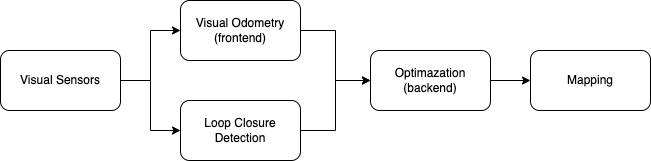
Solution: (SLAM working procedure)

The realtime camera pose and the 3D point cloud are under the world frame, which is usually defined as the camera’s initial pose in real world. In order words, the following camera pose and the 3D point are with respect to this initial camera pose.

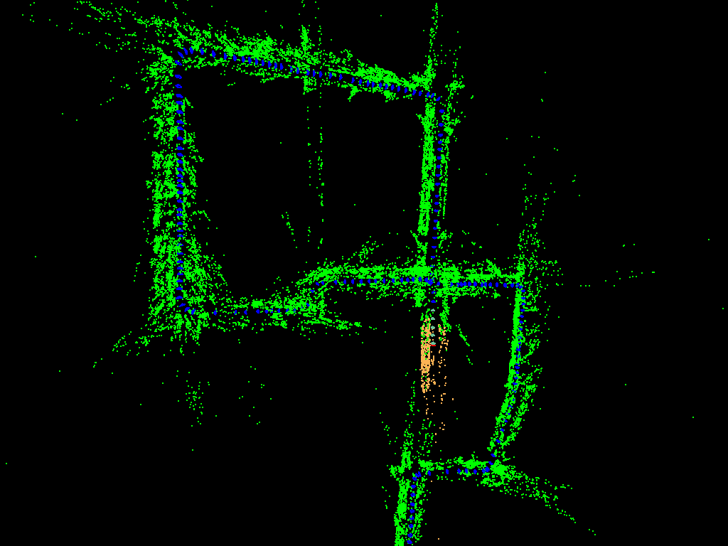
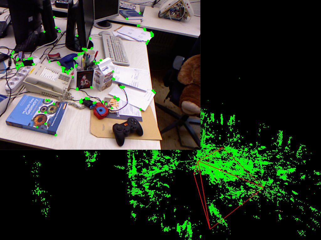
The left image is the reconstructed map of point cloud of KITTI dataset, where green point is the fixed point of street, yellow point is the local point in the map, and blue dots are the previous vehicle’s pose. The right image is the detected keypoint from video stream and the reconstructed map of point cloud of TUM dataset, where the green dots behind is the mappoints of the room, and the red frame represent the camera pose of the current frame.

This post focuses on the SLAM knowledge introduction. For classic SLAM architecture, refer to this post.

Glossary

Click to check

world system, world coordinate system, world frame
- A stationary system fixed in the real world. Usually takes the start position of camera as the origin of world system and front of camera and geomagnetic upper as axises. Coordinate inside this system is called world coordinate.
- Point in world frame, $P_w = [X_w, Y_w, Z_w]^T$
- Several points in world frame, $P_{wj}=[X_{wj}, Y_{wj}, Z_{wj}]^T, j=1,\cdots,n$
camera system, camera coordinate system, camera frame
- A coordinate system attached to the camera and moving with it inside the world frame. Origin is in the light origin of camera, and front is $z$ axis, upper side of camera is $y$ axis. Coordinate inside this frame is called camera coordinate. The third dimension of a space point’s camera coordinate is its depth, which is the distance from the space point to the plane of camera system
- Point under camera frame, $P_c = [X_c, Y_c, Z_c]^T$
- Several points under the same camera frame $P_{cj} = [X_{cj}, Y_{cj}, Z_{cj}]^T, j=1,\cdots,n$
- Point under camera frame $i$, $P_{c_i} = [X_{c_i}, Y_{c_i}, Z_{c_i}]^T, i=1,\cdots,m$
- Point $j$ under camera frame $i$, $P_{c_ij} = [X_{c_ij}, Y_{c_ij}, Z_{c_ij}]^T, i=1,\cdots,m, j = 1,\cdots,n$
- Point in normalized imaging plane, $p_c = [x_c, y_c, 1]^T$
- Point in normalized imaging plane of camera $i$, $p_{c_i} = [x_{c_i}, y_{c_i}, 1]^T, i=1,\cdots,m$
pixel system, pixel coordinate system, pixel frame
- The coordinate system of the capture image. The origin is in the top-left corner and $x$ axis is from left to right, and $y$ axis is from up to down. Coordinate inside this system is called pixel coordinate
- Point in pixel frame, $p = [u, v]^T$
- Point in pixel frame of camera $i$, $p_i = [u_i, v_i]^T, i=1,\cdots,m$
- Point $j$ projecting to camera image $i$, $p_{ij} = [u_{ij}, v_{ij}]^T$, the combination number of $i, j$ is $l \leq mn$
homogeneous coordinate
- Append 1 to point and 0 to vector
- $\mathbf{P}_w$, $\mathbf{p}$
pose, camera extrinsic
- $T_{cw} = \begin{bmatrix} R_{cw} & t_{cw} \\ 0 & 1 \end{bmatrix}$ means transformation of camera frame from world frame
- Transformation of camera $i$ frame from world frame, $T_{c_iw} = \exp(\xi_i^\wedge)$
- Transformation of camera $i$ frame from camera $j$ frame, $T_{c_ic_j}$
camera intrinsic
- $K$, always assumed known
frame, camera image
- The RGB or gray image detected by the camera, usually combing from video stream
keypoint, feature, feature point
- The corners or other special 2D point detected in a frame. In the pixel coordinate
mappoint, space point
- A 3D point in the space. Position fixed in the real world
- Usually in world frame. Can be transformed to the camera frame with camera extrinsic, and then can be transformed to pixel frame with camera intrinsic
map
- A collections of 3D space point. Each space point has a coordinate in world frame
trajectory
- The consistent locations of camera in the space. The location of camera is the translation of the camera
frontend, visual odometry, VO
- Uses to captured frame to calculate pose change of camera, accumulate the pose change to form a trajectory of camera.
- Calculate the world coordinate of nearby space points to establish the local map.
- In generalized meaning, VO also points to the the frontend with a local backend
backend
- Optimization of the poses and world coordinates of mappoints. Usually uses Bundle Adjustment (BA) to optimize all the error terms (constraints). The initial value of estimated target comes from calculated from frontend. Some constraints also comes from loop closure detection.
- Local backend only optimizes nearby important poses and mappoints, while global backend optimizes all important poses and mappoints.

Categories of Visual Sensors

There are several categories of visual sensors, which is the fundamentals and entry point of SLAM. Typically, the RGB image of the environment and the depth (from the camera to the real space position) of each image pixel are required. Stereo (binocular) camera and RGB-D (TOF, structured light) camera could capture the depth image directly, which is the distance from the camera to the target pixel, while Monocular camera can only get the relative distance according to some techniques. Therefore, there will be a scale ambiguity for the monocular SLAM. Different types of visual sensors have different pros and cons.

Name	TOF	Stereo	Structured light	Monocular
Theory	Time of flight, shoot light pulses to the environment and receive the reflection. Then calculate the time between shooting and receiving to get depth	Use 2 camera in a row, according to the difference between 2 images and some already known parameters (distance between 2 cameras), calculate the distance.	Similar to stereo but project infrared speckle encodes to the environment, thus the matching between 2 cameras turns easier	When the object moves, compare the adjacent 2 frames and use the `2D-2D` to get the relative distance to the object. Then uses the triangulation to calculate the depth
Pros	Low calculation power required, high framerate	Less effects from the reflection of the material of object’s surface, longer detection range, higher resolution of the depth image	Faster and more robust in calculation and matching than binocular	Low cost, convenient
Cons	Be affected by the reflection of the material of object’s surface, shorter detection range and lower resolution of the depth image	Required more calculation power for dense map creation	Be affected by the reflection of the material of object’s surface, shorter detection range and lower resolution of the depth image	High calculation power required, Required the camera to move to determine the relative distance, exist scale ambiguity due to no real distance

Camera Basis

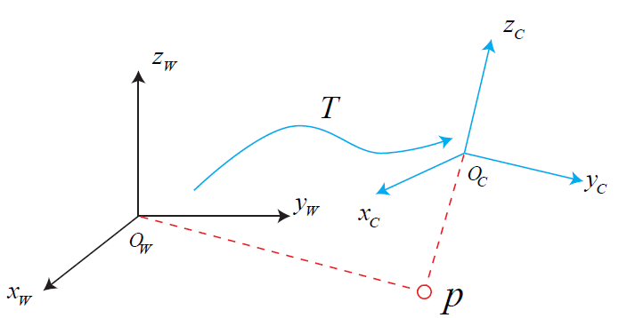
This post uses $T_{cw}$ transformation matrix to describe camera pose. It is to transform any points’ coordinates from world frame $O_w$ to camera frame $O_c$.

For more info about 3D transformation, refer to this post.

Camera imaging model describes the relationship of a 3D point from camera frame (in world units meters), to the imaging frame (in pixels). Pinhole camera is an imaging model for ideal camera, while lens distortion also needs to be consider for real camera.

Pinhole Camera Model

From world frame $P_w$ to camera frame $P_c$ to pixel frame $p$
$$
\begin{split}
Z_c\mathbf{p}=Z_c\begin{bmatrix}
u \\
v \\
1
\end{bmatrix}
=KP_c
&=K(R_{cw}P_w + t_{cw}) \\
&=K(T_{cw}\mathbf{P_w})_{1:3} \\
&=K
\begin{bmatrix}
1 & 0 & 0 & 0 \\
0 & 1 & 0 & 0 \\
0 & 0 & 1 & 0
\end{bmatrix}
T_{cw}\mathbf{P_w}
\end{split}
$$
where

$p$ is the projected point’s pixel coordinate, and $\mathbf{p}$ is the homogeneous form
$P_c=[X_c, Y_c, Z_c]^T$ is the point’s coordinate in camera frame
$Z_c$ is the 3rd dimension of $P_c$, which represents the distance from the point to the camera frame’s coordinate plane
$P_w$ is the point’s coordinate in world frame
$R_{cw}, t_{cw}$ is the camera extrinsic
$K$ is the camera intrinsic
$$K=\begin{bmatrix}
f_x & s & c_x \\
0 & f_y & c_y \\
0 & 0 & 1
\end{bmatrix}
=\begin{bmatrix}
\alpha f & \alpha f \tan(\theta) & c_x \\
0 & \beta f & c_y \\
0 & 0 & 1
\end{bmatrix}$$
where
$f_x, f_y$ is focal length of x / y in pixels
$f$ is focal length in world units, e.g. millimeters
$\alpha, \beta$ is number of pixels in 1 world unit, e.g. pixel / millimeter
$c_x, c_y$ is optical center in pixels
$s$ is skew coefficient, which is non-zero if the image axes are not perpendicular
$\theta$ is the angle of image between vertical axe and the real y axe.

Alternative explanation of above equation

A point with coordinate $P_w$ in world frame
Covert to the camera frame by $P_c = T_{cw}P_w = R_{cw}P_w + t_{cw} = [X_c, Y_c, Z_c]^T$
Project to the camera’s normalized image plane frame (the plane with distance to camera is 1) by $p_c=[\frac{X_c}{Z_c}, \frac{Y_c}{Z_c}, 1]^T$, which is in Homogeneous coordinate
Covert to the pixel coordinate by $\mathbf{p}=Kp_c$ and drop the last dimension to get $p$

Intrinsic analysis

For $P_c^{\prime}$ which in normalized image plane, where the distance to optical origin is 1 world unit. e.g. 1 millimeter

Without the skew, we have the relationship

$$
\frac{X^{\prime}}{1} = \frac{\frac{u}{\alpha}}{f} \rightarrow u = \alpha f X^{\prime} = f_x X^{\prime}
$$

Therefore, focal length x $f_x$ can makes world unit length in normalized plan into respective pixel length.

Due to the skew, horizontal pixel position will change to

$$
u = f_x X^{\prime} + f_x \tan\theta Y^{\prime}
$$

Finally, add the offset in pixels (usually positive scalar)

$$
u = f_x X^{\prime} + s Y^{\prime} + c_x
$$

Distortion

There are radial distortion, caused by light rays bending more near the edges of a lens, and tangential distortion, caused by the lens and the image plane are not parallel.

The relationship between undistorted coordinate in normalized image plane $(X^{\prime}, Y^{\prime})$ and distorted coordinate in normalized image plane $(X_{distorted}^{\prime}, Y_{distorted}^{\prime})$

For radial distortion

$$
\begin{gather}
X_{distorted}^{\prime} = X^{\prime}(1 + k_1 r^2 + k_2 r^4 + k_3 r^6) \\
Y_{distorted}^{\prime} = Y^{\prime}(1 + k_1 r^2 + k_2 r^4 + k_3 r^6)
\end{gather}
$$

For tangential distortion

$$
\begin{gather}
X_{distorted}^{\prime} = X^{\prime} + 2p_1 X^{\prime} Y^{\prime} + p_2 (r^2 + 2 X^{\prime 2}) \\
Y_{distorted}^{\prime} = Y^{\prime} + p_1 (r^2 + 2 Y^{\prime 2}) + 2p_2 X^{\prime} Y^{\prime}
\end{gather}
$$

Usually we make the image undistorted firstly, then we can use the pinhole camera model

In order to establish the relationship between 2 frames or between local map and a frame, the common feature points need to be extracted and matched. This step is also called data association.

Feature Extraction

Feature point in an frame refers to some special pixels, e.g. corner point. Below is some feature point used widely.

Name	keypoint the pixel coordinate of the point, (optional) the direction and scale of the point	Descriptor ID of the keypoint, a vector to describe the nearby pixel info of the keypoint
ORB	`Oriented FAST` 1. Choose a pixel p and the light is $I_p$ 2. Choose a threshold $T$ (e.g. 0.2$I_p$) 3. Traverse the 16 pixels on the circle with p as origin and 3 as radius 4. If there are continuous N (e.g. 12, 9, 11) pixels with light larger than $I_p+T$ or smaller than $I_p-T$, p is the keypoint 5. Use Non-maximal suppression to remove some keypoints in a region 6. Build a feature pyramid to include scale info 7. $\theta=arctan(m_{01}/m_{10})$, where $m_{pq}=\sum_{x,y \in B} x^p y^q I(x,y), p, q = \{0, 1\}$ is the moment of the patch area	`Steer BRIEF (Binary Robust Independent Elementary Feature)` 1. Pick 2 pixels in the patch area near the keypoint p, $p_1=(p_x+dx_1, p_y+dy_1)$, $p_2=(p_x+dx_2, p_y+dy_2)$ 2. Rotate the two points $\theta$ around the point p to get $p_1^{\prime}=(p_x + dx_1 \cos\theta - dy_1 \sin\theta , p_y + dx_1 \sin\theta + dy_1 \cos\theta)$, $p_2^{\prime}=(p_x + dx_2 \cos\theta - dy_2 \sin\theta , p_y + dx_2 \sin\theta + dy_2 \cos\theta)$ 3. get 1 if $I_{p_1^{\prime}}>I_{p_2^{\prime}}$ else 0 4. Do the pick action N (e.g. 128, 256) times to form a $(1\times N)$ 0-1 vector, each time is picking 2 pixels according to the previously random generated results
Harris
Shi-Tomasi
SIFT
FAST
SURF

Feature Matching

Below are two feature matching methods

Feature matching with descriptors
Feature matching with optical flow

For feature points with descriptor, the distance (e.g. Hamming distance, number of different bit) from 2 feature points’ descriptors could be calculated.

Brute-force method will iterative feature points from 2 frames, and calculate their distance, then associate feature points with smallest distance.

Another way is to use FLANN (Fast Library for Approximate Nearest Neighbors). TODO.

Instead of computing descriptors and performing the feature matching, optical flow could directly track motion of the feature points in different frames, saving lots of the time.

Optical flow assumes the gray scale of the corresponding keypoints doesn’t change. If there is a pixel locating in $(x, y)$ in time $t$ and it moves to $(x+\mathrm{d}x, y+\mathrm{d}y)$ in time $t+\mathrm{d}t$, so there is

$$ \begin{aligned}
I(x+\mathrm{d}x, y+\mathrm{d}y, t+\mathrm{d}t)
&= I(x, y, t) \\
&\approx I(x, y, t) + \frac{\partial I}{\partial x}\mathrm{d}x + \frac{\partial I}{\partial y}\mathrm{d}y + \frac{\partial I}{\partial t}\mathrm{d}t
\end{aligned}$$

Therefore, there is
$$\begin{gather}
\frac{\partial I}{\partial x}\mathrm{d}x + \frac{\partial I}{\partial y}\mathrm{d}y = -\frac{\partial I}{\partial t}\mathrm{d}t \\
[I_x, I_y] \begin{bmatrix}
u \\
v
\end{bmatrix} = -I_t
\end{gather}$$
where $I_x, I_y$ are the gradient of the image in horizontal and vertical direction, and $I_t$ is gray scale change. $u, v$ are the moving speed of the pixel.

Supposing a pixel window with size $w\times w$, so there is
$$\begin{bmatrix}
I_{x1} & I_{y1} \\
\vdots & \vdots \\
I_{xw^2} & I_{yw^2}
\end{bmatrix}
\begin{bmatrix}
u \\
v
\end{bmatrix}=
-\begin{bmatrix}
I_{t1} \\
\vdots \\
I_{tw^2}
\end{bmatrix}$$

$u, v$ could be solved by the equations and they represents the new positions of the keypoints after multiplying with time.

Frontend

Input: continuous captured images $I_i, i=1,\cdots,m$
Output
- 6DoF camera pose for each captured frame
- Updated nearby 3D point clouds, or called local map
Solution (monocular, feature-based)
1. Start. At time $t_1$, given image $I_1$
  1. Initialize the $T_{c_1w} = \begin{bmatrix} I_{33} & 0 \\ 0 & 1 \end{bmatrix}$, which means the world frame aligns with the initial camera pose.
2. Initialization. At time $t_2$, given image $I_2$
  1. Extract feature points from $I_1$ and $I_2$, and match the respective feature points.
  2. Use 2D-2D method to solve the relative pose $T_{c_2c_1}=T_{c_2w}$ between 2 frames.
  3. Use triangulation to calculate the 3D position of the matched feature points in world frame from 2 frames, used as the local map.
3. Tracking. At time $t_3, \cdots$
  1. Extract feature points from $I_3$, and match with the local map’s feature points
  2. Use 3D-2D method to solve the relative pose $T_{c_3w}$
  3. Maintain the local map, including deleting some useless mappoints, and adding new mappoints extracted from new images.

An alternative way is to always calculate the relative pose $T_{c_jc_i}$ between 2 frames, then accumulated the pose to get $T_{c_jw} = T_{c_jc_{j-1}}\cdots T_{c_1w}$. This way is simpler but may have more accumulated error it doesn’t consider the common observed features between current frame and other previous frames.

The initialization step is only needed for monocular camera. For stereo and RGBD camera, they could skip it since they could directly know the depth. See following section for more info.

Besides, if using direct method, then the feature matching and geometric solving steps will be replaced by a photometric optimization step to get the extrinsic.

Feature-based Method

Feature based method depends on the matched feature point paris between current frame and previous frames. Usually the camera is already calibrated, meaning the intrinsic is known. The extrinsic could be calculated using following methods.

Methods	First element	Second element	Result
2D-2D	Feature points from last frame	Feature points from current frame	Relative rotation and direction (translation without scale)
3D-2D	Mappoints in last frame’s camera coordinate, or world frame	Feature points of current frame	Relative pose change from last frame, or world pose of current frame
3D-3D	Mappoints in last frame’s camera coordinate, or world frame	Mappoints in last frame’s camera coordinate	Relative pose change from last frame, or world pose of current frame

More explanation

For monocular camera, it knows nothing about any mappoints at the beginning. Therefore, it needs initialization to build the initial map. This initialization is using the 2D-2D method based on different frames to calculate the relative pose changes, and then triangulate the feature points to calculate the respective mappoints. Once this initial map is built, following frames could use 3D-2D method to estimate the pose from the map.

For the stereo and RGBD camera, they could get the depth information at the beginning (stereo camera could uses 2 cameras to triangulate feature points to get the respective mappoints, RGBD could directly get the depth), so they can easily build the initial map. For the following frame, they could know directly of the respective mappoints of extracted feature points, so they could perform 3D-3D pose estimation. However, it waste time for the stereo camera to do extra extraction of feature points and feature matching between left and right frames, so stereo usually uses 3D-2D for pose estimation.

For RGBD camera, some feature points may not have depth measurement due to noise, so a BA combines 3D-3D (for feature points have depth), and 3D-2D (for feature points without depth) is used to do pose estimation.

2D-2D: Epipolar Constraint

Input: Matched 2-d keypoint pairs from 2 images
- $p_{1j} = [u_{1j}, v_{1j}]^T, j=1,\cdots,n$ in pixel coordinate
- $p_{2j} = [u_{2j}, v_{2j}]^T, j=1,\cdots,n$ in pixel coordinate
Output: $T_{c_2c_1}$ up to scale
Solution
1. Use matched keypoint pairs to calculate one of the following matrix
2. Calculate $R$, $t$ from the matrix

Matched keypoint pairs have the following equations, notice here we just use 1 matched pair.

Matrix	Equations	Matrix DoF	Required minimal pairs	Constraints
Fundamental matrix $F$	$\mathbf{p}_2^T F \mathbf{p}_1 = 0$	8	8	Cannot recover $R$, $t$ for pure rotation scenario
Essential matrix $E$	$\mathbf{p}_{c_2}^T E \mathbf{p}_{c_1}$	5	5	Cannot recover $R$, $t$ for pure rotation scenario
Homography matrix $H$	$\mathbf{p}_2 = H\mathbf{p}_1$	8	4	Need points in same plane or very far away

Fundamental and Essential Matrix
Homography Matrix

Definition

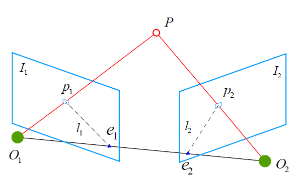
For 1 matched pair, according to the spatial geometry, we know the vector $O_1O_2$, $O_2P$, and $O_1P$ are coplanar, so we have.

$$
\begin{split}
& (O_1O_2 \times O_2P) \cdot O_1P = 0 \\
\Rightarrow & (t_{c_2c_1} \times K^{-1}\mathbf{p}_2) \cdot (R_{c_2c_1} K^{-1}\mathbf{p}_1) = 0 \\
\Rightarrow & (t_{c_2c_1}^\wedge K^{-1}\mathbf{p}_2)^T (R_{c_2c_1} K^{-1}\mathbf{p}_1) = 0 \\
\Rightarrow & \mathbf{p}_2^T K^{-T} t_{c_2c_1}^\wedge R_{c_2c_1} K^{-1} \mathbf{p}_1 = 0 \\
\Rightarrow & \mathbf{p}_2^T F \mathbf{p}_1 = 0 \\
\Rightarrow & \mathbf{p}_{c_2}^T E \mathbf{p}_{c_1} = 0
\end{split}
$$
where
$$
F=K^{-T} t_{c_2c_1}^\wedge R_{c_2c_1} K^{-1}, \quad
E=t_{c_2c_1}^\wedge R_{c_2c_1}
$$

$\mathbf{p}_1$, $\mathbf{p}_2$ are the pixel coordinate of keypoint in homogeneous coordinate
$\mathbf{p}_{c_1}=K^{-1}\mathbf{p}_1$, $\mathbf{p}_{c_2}=K^{-1}\mathbf{p}_2$ are 3D coordinate of feature point in the normalized image plane, which is also the vector from camera origin through that feature point and expressed under each camera frame
$F$ is fundamental matrix
$E$ is essential matrix
$R_{c_2c_1}$, $t_{c_2c_1}$ is the camera extrinsic we want to solve

Calculate matrix

Therefore, if we know the camera intrinsic, we could calculate the essential matrix using all the matched point pairs by constructing the functions as $[\mathbf{p}_{21}, \cdots, \mathbf{p}_{2n}]^T E [\mathbf{p}_{11}, \cdots, \mathbf{p}_{1n}] = 0$, which eventually could be wrote as the form of homogeneous linear equations $AX = 0$. Since 1 pair contribute to 1 constraint of $E$, and $E$ has 5 DoF, so we need at least 5 feature point pairs to solve $E$. (could also use 8 pairs for easier calculation).

If we don’t know the camera intrinsic, we could calculate the fundamental matrix $F$, which requires 8 feature point pairs, and recover $K$, $R$, $t$ from $F$.

Calculate $R$, $t$

Perform SVD for matrix $E$, where $E = U \Sigma V^T$
Enforce the singular values to be 1 to meet the essential matrix constraints, where
$$
E^\prime = U \begin{bmatrix}
1 & 0 & 0 \\
0 & 1 & 0 \\
0 & 0 & 0
\end{bmatrix}
V^T
= U \begin{bmatrix}
0 & 1 & 0 \\
-1 & 0 & 0 \\
0 & 0 & 0
\end{bmatrix}
\begin{bmatrix}
0 & -1 & 0 \\
1 & 0 & 0 \\
0 & 0 & 0
\end{bmatrix}
V^T
$$
Calculate 4 potential results of $R$ and $t$ by
$$
\begin{aligned}
t_1^{\wedge} = \pm U
\begin{bmatrix}
0 & -1 & 0 \\
1 & 0 & 0 \\
0 & 0 & 1
\end{bmatrix}
U^T, \quad
R_1 = U
\begin{bmatrix}
0 & 1 & 0 \\
-1 & 0 & 0 \\
0 & 0 & 1
\end{bmatrix}
V^T
\\
t_2^{\wedge} = \pm U
\begin{bmatrix}
0 & 1 & 0 \\
-1 & 0 & 0 \\
0 & 0 & 1
\end{bmatrix}
U^T, \quad
R_2 = U
\begin{bmatrix}
0 & -1 & 0 \\
1 & 0 & 0 \\
0 & 0 & 1
\end{bmatrix}
V^T
\end{aligned}
$$
Use the 4 combinations of $R$, $t$ to calculate the distance of the space point. Select the only 1 combination with the distance larger than 0
Normalize the $t$ to initialize the scale (Later, the unit is the real length of $t$.)

Definition

For a common point under 2 cameras, there are
$$
\begin{aligned}
& Z_{c_1} \mathbf{p}_1 = K P_{c_1} \\
& Z_{c_2} \mathbf{p}_2 = K (R_{c_2c_1} P_{c_1} + t_{c_2c_1})
\end{aligned}
$$
where $P_{c_1}$ is the coordinate of mappoint under camera $1$ frame.

If all the matched feature points are in the same physical plane or they are very far away (in the infinity plane), we could assume the plane equation is
$$
\begin{aligned}
& n^T P_{c_1} + d = 0 \\
\Rightarrow & -\frac{n^T P_{c_1}}{d} = 1
\end{aligned}
$$

So we have
$$
\begin{split}
Z_{c_2} \mathbf{p}_2
&= K (R_{c_2c_1} P_{c_1} + t_{c_2c_1}) \\
&= K (R_{c_2c_1} P_{c_1} - t_{c_2c_1}\frac{n^T P_{c_1}}{d}) \\
&= K (R_{c_2c_1} - \frac{t_{c_2c_1} n^T}{d}) P_{c_1} \\
&= Z_{c_1} K (R_{c_2c_1} - \frac{t_{c_2c_1} n^T}{d}) K^{-1} \mathbf{p}_1 \\
\Rightarrow & \quad \mathbf{p}_2 = H \mathbf{p}_1
\end{split}
$$
where
$$
H = K (R_{c_2c_1} - \frac{t_{c_2c_1} n^T}{d}) K^{-1}
$$
is a $3\times 3$ matrix and up to scale.

Calculate matrix

Therefore, if we know the camera intrinsic, we could calculate the essential matrix using the matched feature point pair by constructing the functions as $[\mathbf{p}_{21}, \cdots, \mathbf{p}_{2n}] = H [\mathbf{p}_{11}, \cdots, \mathbf{p}_{1n}]$, which eventually could be wrote as the form of homogeneous linear equations $AX = 0$. Since 1 pair contribute to 2 constraint of $E$, and $H$ has 8 DoF, so we need at least 4 feature point pairs to solve $H$.

Calculate $R$, $t$

Perform SVD for $H$, where $H = \begin{bmatrix} h_1 & h_2 & h_3 \end{bmatrix} = U\Sigma V^T$
They we have
$$
R = U \begin{bmatrix}
1 & 0 & 0 \\
0 & 1 & 0 \\
0 & 0 & \det (UV^T)
\end{bmatrix} V^T, \quad
t = \frac{h_3}{||h_1||}
$$

Triangulation

Input:
- 1 matched 2-d keypoint pair $p_i=[u_i, v_i]^T, i=1,\cdots,m$ from at least 2 images
- Respective camera pose $T_{c_iw}$
Output: 3D position $P_w=[X_w, Y_w, Z_w]^T$ of mappoint projecting to those keypoints
Solution:

General Scenario
Parallel Stereo Cameras Scenario

From the camera imaging model of this mappoint on camera $i$, we have
$$
\begin{split}
&Z_{c_i} \begin{bmatrix}
u_i \\
v_i \\
1
\end{bmatrix} =
K
\begin{bmatrix}
1 & 0 & 0 & 0 \\
0 & 1 & 0 & 0 \\
0 & 0 & 1 & 0
\end{bmatrix}
T_{c_i w}
\begin{bmatrix}
X_w \\
Y_w \\
Z_w \\
1
\end{bmatrix} \\
\Rightarrow&
\begin{bmatrix}
Z_{c_i} u_i \\
Z_{c_i} v_i \\
Z_{c_i}
\end{bmatrix}
=
P_i
\begin{bmatrix}
X_w \\
Y_w \\
Z_w \\
1
\end{bmatrix}
=
\begin{bmatrix}
P_{i1} \\
P_{i2} \\
P_{i3}
\end{bmatrix}
\begin{bmatrix}
X_w \\
Y_w \\
Z_w \\
1
\end{bmatrix}
\end{split}
$$
where

$P_i \in \mathbb{R}^{3\times 4}$, and $P_{i1}, P_{i2}, P_{i3}$ are the rows
$Z_{c_i}$ is the distance of mappoint in camera frame $i$

Bringing the 3rd equation to the first 2 could get
$$
\begin{split}
&\begin{bmatrix}
u_i P_{i3} \mathbf{P}_w\\
v_i P_{i3} \mathbf{P}_w
\end{bmatrix} =
\begin{bmatrix}
P_{i1} \mathbf{P}_w\\
P_{i2} \mathbf{P}_w
\end{bmatrix} \\
\Rightarrow&
\begin{bmatrix}
u_i P_{i3} - P_{i1} \\
v_i P_{i3} - P_{i2}
\end{bmatrix}
\mathbf{P}_w = 0
\end{split}
$$
where $\mathbf{P}_w$ is the homogeneous coordinate of the mappoint.

Since $\mathbf{P}_w$ has 3DoF, and each keypoint provides 2 constraints. Thus we need at least 2 keypoints from different images to solve the 3D position of mappoint. The more equations, the more accurate result we could get. The equations is in the form of $AX=0$ and can be solved by SVD.

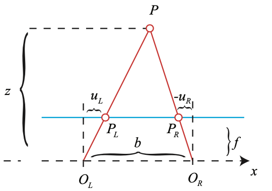
If there are 2 parallel cameras whose distance $b$ is already known, when there are 2 matched keypoint $p_L=p_1$ from left image and $p_R=p_2$ from right image, the depth $z$ of the mappoint could be calculated as following.

$$
\begin{split}
&\frac{z-f}{z} = \frac{b-(u_L - u_R)}{b} \\
\Rightarrow& z = \frac{b}{u_L - u_R} f
\end{split}
$$
where

$u_L = (f K^{-1} \mathbf{p}_1)_{:1}$ is the 1st of keypoint $p_L$ in the focal plane in camera frame
$u_R = (f K^{-1} \mathbf{p}_2)_{:1}$ is the 1st of keypoint $p_R$ in the focal plane in camera frame
$f$ is the focal length in meter

The maximum depth of this parallel stereo camera setup could measure is $bf$.

3D-2D: PnP

Perspective-n-point

Input: Matched point pairs from 3D map (or previous camera frame) and image
- 3-d mappoint $P_{wj} = [X_{wj}, Y_{wj}, Z_{wj}]^T,j=1,\cdots,n$ in world frame
- 2-d keypoint $p_{ij}=[u_{ij}, v_{ij}]^T,j=1,\cdots,n$ in pixel coordinate of camera $i$, note $i$ is fixed here
Output: $T_{c_iw}$
Solution:

Definition

For 1 matched point pair
$$
Z_c\begin{bmatrix}
x_c \\
y_c \\
1
\end{bmatrix}
=[R_{cw} | t_{cw}]P_w
=M P_w
=\begin{bmatrix}
t_1 & t_2 & t_3 & t_4 \\
t_5 & t_6 & t_7 & t_8 \\
t_9 & t_{10} & t_{11} & t_{12}
\end{bmatrix}
\begin{bmatrix}
X_w \\
Y_w \\
Z_w \\
1
\end{bmatrix}
$$
where

$Z_c$ is the distance from camera to the space point
$M\in \mathbb{R}^{3\times 4}$
$[x_c, y_c, 1]^T$ is the coordinate of the mappoint in normalized plane, can could be calculated by
$$
\begin{bmatrix}
x_c \\
y_c \\
1
\end{bmatrix} = K^{-1}
\begin{bmatrix}
u \\
v \\
1
\end{bmatrix}
$$

By bring the 3rd equation to above 2 and after some operations, we could get
$$
\begin{bmatrix}
P_{w}^T & 0 & -x_{c}P_{w}^T \\
0 & P_{w}^T & -y_{c}P_{w}^T
\end{bmatrix}
\begin{bmatrix}
t_1 \\ t_2 \\ t_3 \\ t_4 \\ t_5 \\ t_6 \\ t_7 \\ t_8 \\ t_9 \\ t_{10} \\ t_{11} \\ t_{12}
\end{bmatrix} = 0
$$

Calculate matrix

Since matrix $M$ has 12 DoF, and each matched pair contributes to 2 constraints, we need at least 6 matched pair to solve the equations in the form $AX=0$.

Calculate $R$, $t$

Since $M = [R | t]$, then $t$ is directly the last column of matrix $M$
The $R$ extracted from $M$ may not meet the requirement of $SO(3)$, so we use the following equation to estimate the $R^\prime$
$$
R^\prime = (RR^T)^{-\frac{1}{2}}R
$$

Definition

For 3 space points $A, B, C$, the relationships between their coordinates in normalized plane $p_{c_A}, p_{c_B}, p_{c_C}$ and camera frame $P_{c_A}, P_{c_B}, P_{c_C}$ could be used similar triangle to come up with following equations

$$
\begin{aligned}
&(1-u)y^2 - ux^2 - \cos\langle b, c \rangle y + 2uxy\cos\langle a, b \rangle + 1 = 0 \\
&(1-w)x^2 - wy^2 - \cos\langle a, c \rangle x + 2wxy\cos\langle a, b\rangle + 1 = 0
\end{aligned}
$$
where

$u = \frac{BC^2}{AB^2}$, $w = \frac{AC^2}{AB^2}$ could be given by their coordinate in world frame $P_{w_A}, P_{w_B}, P_{w_C}$ since the fraction of length don’t change under world frame or camera frame
$x = \frac{OA}{OC}$, $y = \frac{OB}{OC}$ need to be solved

Solve equations

The equations will have up to 4 solutions, and we need to use an additional point to verify which solution is correct. So this method requires at least 3 point.

Calculate $R$, $t$

Solve above equations to get length of $OA$, $OB$, and $OC$
Get the points coordinate under camera frame $P_{cA}, P_{cB}, P_{cC}$
Use 3D-3D to solve $R$, $t$ from $P_{wA}, P_{wB}, P_{wC}$ and $P_{cA}, P_{cB}, P_{cC}$

Optimization target

DLT and P3P only use several matched point pairs, while BA put all matched point pairs together to build an optimization target to minimize the reprojection error. It’s more accurate but requires a good initial value from DLT or P3P since it needs to be solved by iterative method.

The difference between this frontend 3D-2D BA and the backend BA is that this frontend BA only optimizes the camera pose in the optimization target but keeps the mappoints position fixed.

For the space points in world coordinate $P_{wj}=[X_{wj}, Y_{wj}, Z_{wj}]^T$ and their respective pixel coordinates of camera $i$, $p_{ij}=[u_{ij}, v_{ij}]^T$, and $j=1,\cdots,n$, we have
$$
Z_{c_ij}\mathbf{p}_{ij} = K(T_{c_iw}\mathbf{P}_{wj})_{1:3},\quad j=1,\cdots,n
$$

So we could have the optimization target
$$
\begin{split}
T_{cw}^{*}
&= \mathrm{arg} \min_{T_{cw}} \frac{1}{2} \sum_{j=1}^n
\begin{Vmatrix}
e_j
\end{Vmatrix}^2 \\
&= \mathrm{arg} \min_{T_{cw}} \frac{1}{2} \sum_{j=1}^n
\begin{Vmatrix}
p_{ij}-\frac{1}{Z_{c_ij}}
\left( K (T_{c_iw} \mathbf{P}_{wj})_{1:3} \right)_{1:2}
\end{Vmatrix}^2 \\
&= \mathrm{arg} \min_{T_{cw}} \frac{1}{2} \sum_{i=1}^n
\begin{Vmatrix}
\begin{bmatrix}
u_{ij} - (f_x \frac{X_{c_ij}}{Z_{c_ij}} + c_x) \\
v_{ij} - (f_y \frac{Y_{c_ij}}{Z_{c_ij}} + c_y)
\end{bmatrix}
\end{Vmatrix}^2
\end{split}
$$
where

$P_{c_ij} = [X_{c_ij}, Y_{c_ij}, Z_{c_ij}]^T = (T_{c_iw} \mathbf{P}_{wj})_{1:3}$ is the coordinate of mappoint in camera frame
$Z_{c_ij}$ is the 3rd dimension of point $P_{c_ij}$

Solve $T$

In reality, we will write the optimization into matrix form instead of sum form, and use Lie Algebra to represent the camera pose, then use iterative method to solve it. See more details in backend section.

Here we just simply give the Jocobian matrix of $e_i$ on camera pose $\xi=\ln(T_{cw})^\vee$, which will be used to calculate the $\Delta \xi$ for reach iteration.
$$
\begin{split}
\frac{\partial e_i}{\partial \xi}
&= \frac{\partial e_i}{\partial P_{c_ij}} \frac{\partial P_{c_ij}}{\partial \xi} \\
&= -\begin{bmatrix}
\frac{f_x}{Z_{c_ij}} & 0 & -\frac{f_x X_{c_ij}}{(Z_{c_ij})^2} & -\frac{f_x X_{c_ij} Y_{c_ij}}{(Z_{c_ij})^2} & f_x+\frac{f_x(X_{c_ij})^2}{(Z_{c_ij})^2} & -\frac{f_x Y_{c_ij}}{Z_{c_ij}} \\
0 & \frac{f_y}{Z_{c_ij}} & -\frac{f_y Y_{c_ij}}{(Z_{c_ij})^2} & -f_y - \frac{f_y(Y_{c_ij})^2}{(Z_{c_ij})^2} & \frac{f_y X_{c_ij} Y_{c_ij}}{(Z_{c_ij})^2} & \frac{f_y X_{c_ij}}{Z_{c_ij}}
\end{bmatrix}
\end{split}
$$

Note that in some implementation like Sophus::SE3d where the $\xi_0, \xi_1, \xi_2$ represents the translation, and $\xi_3, \xi_4, \xi_5$ represents the rotation, the Jocobian form is like above. However for some implementation like g2o::SE3Quat, where the first 3 elements represent the rotation, then the columns of the Jacobian matrix should switch.

3D-3D: ICP

Iterative Closest Point

ICP is a method common used in Lidar SLAM, where the captured 3D point by Lidar don’t have descriptors, so the procedure to calculate the $R$, $t$ between 2 groups of 3D points are

Choose the closet point from 2 groups to be the matched point pair
Calculate the $R$, $t$ based on the matched point pairs
Transform the one group of points, and repeat step 1-2 until the matched point pair don’t change

Since the visual SLAM could calculate the matched point pair, so the iterative steps could be skipped, and this section only focuses on the calculation of step 2.

Input: Matched 3-d mappoint point pairs from 3D map (or previous camera frame) and camera frame (or another 3D map)
- $P_{wj} = [X_{wj}, Y_{wj}, Z_{wj}]^T, j=1,\cdots,n$ in world frame
- $P_{cj}=[X_{cj}, Y_{cj}, Z_{cj}]^T, j=1,\cdots,n$ in camera frame
Output: $T_{cw}$
Solution:

SVD
BA (Bundle Adjustment)

Optimization target

For the matched 3-d feature point pairs
$$
P_{cj} = R_{cw} P_{wj} + t_{cw}, \quad j=1,\cdots,n
$$
So we have the optimization target
$$
(R^{*},t^{*})=\arg \min_{R,t} \frac{1}{2}\sum_{i=1}^n
\begin{Vmatrix}P_{cj}-(RP_{wi}+t)\end{Vmatrix}^2
$$

Simplify

Defining
$$
P_c^\prime = \frac{1}{n} \sum_{j=1}^n P_{cj}, \quad
P_w^\prime = \frac{1}{n} \sum_{j=1}^n P_{wj}
$$

Then
$$
\begin{split}
\frac{1}{2}\sum_{j=1}^n
\begin{Vmatrix}
P_{cj} - (RP_{wi}+t)
\end{Vmatrix}^2
&=\frac{1}{2}\sum_{j=1}^n\begin{Vmatrix}
P_{cj} - P_c^\prime + P_c^\prime - RP_{wi} -RP_w^\prime + RP_w^\prime - t
\end{Vmatrix}^2 \\
&=\frac{1}{2}\sum_{j=1}^n\begin{Vmatrix}
P_{cj} - P_c^\prime - R(P_{wj} - P_w^\prime) + P_c^\prime - RP_w^\prime - t
\end{Vmatrix}^2 \\
&=\frac{1}{2}\sum_{j=1}^n \left(
\begin{Vmatrix}
P_{cj} - P_c^\prime - R(P_{wj} - P_w^\prime)
\end{Vmatrix}^2 +
\begin{Vmatrix}
P_c^\prime - RP_w^\prime - t
\end{Vmatrix}^2 \right. \\
&\left. \quad + 2\begin{Vmatrix}
P_{cj} - P_c^\prime - R(P_{wj} - P_w^\prime)
\end{Vmatrix}
\begin{Vmatrix}
P_c^\prime - RP_w^\prime - t
\end{Vmatrix}
\right) \\
&=\frac{1}{2}\sum_{j=1}^n \left(
\begin{Vmatrix}
P_{cj} - P_c^\prime - R(P_{wj} - P_w^\prime)
\end{Vmatrix}^2 +
\begin{Vmatrix}
P_c^\prime - RP_w^\prime - t
\end{Vmatrix}^2 \right) \\
&=\frac{1}{2}\sum_{j=1}^n \left(
\begin{Vmatrix}
Q_{cj} - RQ_{wj}
\end{Vmatrix}^2 +
\begin{Vmatrix}
P_c^\prime - RP_w^\prime - t
\end{Vmatrix}^2 \right)
\end{split}
$$
where

$Q_{cj} = P_{cj} - P_c^\prime, j=1,\cdots,n$
$Q_{wj} = P_{wj} - P_w^\prime, j=1,\cdots,n$

Using the first term could get $R$, and then using the second term could get $t$

Solve for $R$, $t$

Construct
$$
W = \sum_{j=1}^n Q_{cj} Q_{wj}^T
$$
Perform SVD for $W$, where $W = U\Sigma V^T$
$R = UV^T$
$t = P_c^\prime - RP_w^\prime$

Optimization target

From the same optimization target
$$
(R^{*},t^{*})
=\arg \min_{R,t} \frac{1}{2}\sum_{j=1}^n
\begin{Vmatrix}
e_j
\end{Vmatrix}^2
=\arg \min_{R,t} \frac{1}{2}\sum_{j=1}^n
\begin{Vmatrix}
P_{cj}-(R_{cw}P_{wj}+t_{cw})
\end{Vmatrix}^2
$$
Use Lie algebra for the optimization target, we could get
$$
\xi^{*} = \arg \min_{\xi} \frac{1}{2} \sum_{j=1}^n
\begin{Vmatrix}
(P_{cj} - (\exp(\xi^{\wedge})P_{wj})_{1:3})
\end{Vmatrix}^2
$$

Solve $T$

Similar to the 3D-2D BA, this optimization will be wrote as matrix form, and only optimize the camera pose. The Jocobian matrix of $e_i$ on camera pose $\xi$ is
$$
\frac{\partial e_j}{\partial \xi^T}
= \frac{\partial e_j}{\partial (\exp(\xi^{\wedge})P_{wj})_{1:3}^T} \frac{\partial (\exp(\xi^{\wedge})P_{wj})_{1:3}}{\partial \xi^T} = -[I_{33} \quad -(R_{cw} P_{wj} + t_{cw})^{\wedge}] \in \mathbb{R}^{3\times 6}
$$

See more details about the optimization in backend part.

3D-3D BA usually used together with 3D-2D BA for RGBD cameras since sometimes not all the depth of pixel could be got in the cameras, for those points, the 3D-2D relationships need to be used.

Direct Method

Input: 2 frames
Output: $T_{c_2c_1}$ between 2 frames
Solution: minimizing the photometric error

Different like feature-based method depends on minimizing the geomagnetic error of feature points to estimate pose, direct method estimate the pose directly by minimizing the photometric error, saving time to extract features, descriptors, and feature matching.

Direct method is similar to the optical flow, while the optical flow computes the feature points motion, while direct method estimates the relative pose change.

Backend

The frontend only optimizes 1 camera pose, while the mappoint positions also have errors, which makes the following camera pose accumulate more and more errors. To make the whole system more accurate and geometric consistency, backend is needed to optimize both camera poses and mappoint positions.

If only several camera poses are involved in backend, it’s called filter method or local optimization. While if all camera poses are involved, it’s called global optimization.

Input: observations from camera pose and mappoint
- Frame poses $T_{c_iw}=\exp(\xi_i^\wedge), i=1,2,\cdots,m$ (usually are keyframes instead of normal frames)
- 3-d mappoint positions $P_{wj}=[X_{wj}, Y_{wj}, Z_{wj}]^T, j=1,2,\cdots,n$ in world frame
- 2-d keypoint $p_{ij}=[u_{ij}, v_{ij}]^T$ of point $j$ projecting into image $i$ in pixel coordinate. Totally $l \leq mn$ number of unique keypoints
Output
- Revised frame poses $T_{c_iw}, i=1,2,\cdots,m$
- Revised frame 3-d mappoint positions $P_{wj}, j=1,2,\cdots,n$ in world frame
Solutions: Filter method, or optimization method to minimize the reprojection error
1. Reads data with noise from frontend and data from loop closure detection
2. Optimizes the camera poses and mappoint positions

Filter method	Optimization method
Incremental method	Batch method
Maintain an estimation of current state, then use new input and system equations to estimate of the next state, and use new observation to refine it	Use all data from time $0$ to time $k$, to estimate the whole state from time $0$ to time $k$ by maximizing the posterior probability of state.
Representative: EKF (Extended Kalman Filter)	Representative: Graph Optimization
MAP (Maximize a Posterior)	MAP (Consider input and system equations) or MLE (Maximize Likelihood Estimation, only consider observations)

Optimization method is considered better than filter these days since it uses more data and could optimize in a large extent.

Filter Method

Extended Kalmal filter method, relevant info could be found in this post.

Optimization Method

The optimization method is to construct a least square optimization target using several camera poses and mappoint positions, and use iterative method to solve it. It is a batch estimation, or called Bundle Adjustment.

This section mainly talks about the final forms of the optimization. Refers to this post for more details of least square and iterative optimization methods.

Build Optimization Target (Cost Function)

The error function for the one of the observations is
$$
\begin{split}
e_{ij}
&=p_{ij}-h(T_{c_iw}, P_{wj}) \\
&=p_{ij}-
\left(
\frac{1}{Z_{c_ij}}K(T_{c_iw}\mathbf{P}_{wj})_{1:3}
\right) _{1:2} \\
&=p_{ij}-
\left(
\frac{1}{Z_{c_ij}}K(R_{c_iw}P_{wj}+t_{c_iw})
\right) _{1:2} \\
&=p_{ij}-
\left(
\frac{1}{Z_{c_ij}} K P_{c_ij}
\right) _{1:2} \\
&=\begin{bmatrix}
u_{ij} \\
v_{ij}
\end{bmatrix} -
\left(\frac{1}{Z_{c_ij}}
\begin{bmatrix}
f_x & 0 & c_x \\
0 & f_y & c_y \\
0 & 0 & 1
\end{bmatrix}
\begin{bmatrix}
X_{c_ij} \\
Y_{c_ij} \\
Z_{c_ij}
\end{bmatrix}
\right) _{1:2} \\
&=\begin{bmatrix}
u_{ij} - (f_x \frac{X_{c_ij}}{Z_{c_ij}} + c_x) \\
v_{ij} - (f_y \frac{Y_{c_ij}}{Z_{c_ij}} + c_y)
\end{bmatrix}
\in \mathbb{R}^{2}
\end{split}
$$
where

$T_{c_iw} =
\begin{bmatrix}
R_{c_iw} & t_{c_iw} \\
0 & 1
\end{bmatrix}$ is the camera pose $i$
$P_{c_ij}=[X_{c_ij}, Y_{c_ij}, Z_{c_ij}]^T$ is position coordinate of mappoint $j$ in camera $i$ frame

The optimization target is the sum of all observation error functions, which is
$$
\frac{1}{2}\sum\limits_{i, j}^l e_{ij}^T \Omega_{i, j} e_{i,j}
$$
where $\Omega_{i, j} \in \mathbb{R}^{2\times 2}$ is called information matrix, which is the inverse of the covariance matrix of the observation noise.

In practice, we usually stack all the state variables together and use the matrix form by

Use the Lie Algebra form $\xi_i=\ln(T_{c_iw})^\vee$ to represent the camera pose
Stacking all states to be estimated together as one vector
$$
x= \begin{bmatrix}
\xi_1 \\
\xi_2 \\
\vdots \\
\xi_m \\
P_{w1} \\
P_{w2} \\
\vdots \\
P_{wn}
\end{bmatrix} \in \mathbb{R}^{6m + 3n}
$$
Stack all the error terms together to be
$$
f(x) = \begin{bmatrix}
e_{11} \\
e_{14} \\
\vdots \\
e_{ij} \\
\vdots \\
e_{mn}
\end{bmatrix} \in \mathbb{R}^{2l}
$$
where $l$ is the number of observations
Stack all the information matrix together to be
$$
\Omega = \begin{bmatrix}
\Omega_{11} & \cdots & \cdots \\
\cdots & \Omega_{ij} & \cdots \\
\cdots & \cdots & \Omega_{mn}
\end{bmatrix} \in \mathbb{R}^{2l \times 2l}
$$
The optimization target turns to
$$
x^* = \arg\min_x \frac{1}{2} f(x)^T \Omega f(x)
$$

In g2o library implementation

Get keyframes and respective mappoints from frontend
Form the optimization problem
- g2o library uses a graph optimization structure
- Create several pose vertexes representing the poses, set the value from frontend as the initial value
- Create several mappoint vertexes representing the mappoints, set the value from frontend as the initial value
- Build several binary edges with 2-d keypoints pixel coordinates as measurement
- Link every edge to the two corresponding vertex
Iterate to get the updated values of camera poses and mappoint positions

Solve the Least Square Problem

The optimization target is an non-linear least square problem, so we need to use iterative local linearization methods to solve it, which is

Use the values from frontend as the initial guess $x_0$
Calculate $\Delta x$ at each step, to update state vector by $x_k + \Delta x \rightarrow x_{k+1}$

This section takes the Gauss-Newton optimization method as example. More iterative methods could be found here.

At position $x_k$, the nearby cost function is (note $x_k$ is known and $\Delta x$ is unknown)

$$
\frac{1}{2} f(x_k+\Delta x)^T \Omega f(x_k+\Delta x) \approx \frac{1}{2} (f(x_k) + J\Delta x)^T \Omega (f(x_k) + J\Delta x)
$$
where
$$
\begin{split}
J
&= \left. \frac{\mathrm{d} f(x)}{\mathrm{d} x^T} \right|_{x_k} \\
&= \begin{bmatrix}
F \ | \ E
\end{bmatrix} \\
&= \begin{bmatrix}
F_{11} & \cdots & 0 & E_{11} & \cdots & 0 \\
F_{14} & \cdots & 0 & 0 & E_{14} & \cdots \\
\vdots & \vdots & \vdots & \vdots & \vdots & \vdots \\
\cdots & F_{ij} & \cdots & \cdots & E_{ij} & \cdots \\
\vdots & \vdots & \vdots & \vdots & \vdots & \vdots
\end{bmatrix}
\in \mathbb{R}^{2l \times (6m+3n)}
\end{split}
$$
where

$J \in \mathbb{R}^{2l \times (6m+3n)}$ is the Jacobian matrix of concatenated error function $f(x) \in \mathbb{R}^{2l}$ on the concatenated state vector $x \in \mathbb{R}^{6m+3n}$
$F \in \mathbb{R}^{2l \times 6m}$ is the Jacobian matrix of concatenated error function $f(x)$ on the concatenated state vector of camera poses $[\xi_1, \xi_2, \cdots, \xi_m]^T \in \mathbb{R}^{6m}$
$E \in \mathbb{R}^{2l \times 3n}$ is the Jacobian matrix of concatenated error function $f(x)$ on the concatenated state vector of mappoint position $[P_{w1}, P_{w2}, \cdots, P_{wn}]^T \in \mathbb{R}^{3n}$
$F_{ij} \in \mathbb{R}^{2 \times 6}$ is the Jacobian matrix of error term $e_{ij} \in \mathbb{R}^{2}$ on the camera pose $\xi_i \in \mathbb{R}^{6}$, which is
$$
\begin{split}
F_{ij} = \frac{\partial e_{ij}}{\partial \xi_i^T}
&= \frac{\partial e_{ij}}{\partial P_{c_ij}^T}\frac{\partial P_{c_ij}}{\partial \xi_i^T} \\
&= -\begin{bmatrix}
\frac{f_x}{Z_{c_ij}} & 0 & -\frac{f_x X_{c_ij}}{(Z_{c_ij})^2} \\
0 & \frac{f_y}{Z_{c_ij}} & -\frac{f_y Y_{c_ij}}{(Z_{c_ij})^2}
\end{bmatrix}
\begin{bmatrix}
I_{33} & -(R_{c_iw}P_{wj}+t_{c_iw})^{\wedge}
\end{bmatrix} \\
&= -\begin{bmatrix}
\frac{f_x}{Z_{c_ij}} & 0 & -\frac{f_x X_{c_ij}}{(Z_{c_ij})^2} \\
0 & \frac{f_y}{Z_{c_ij}} & -\frac{f_y Y_{c_ij}}{(Z_{c_ij})^2}
\end{bmatrix}
\begin{bmatrix}
1 & 0 & 1 & 0 & Z_{c_ij} & -Y_{c_ij} \\
0 & 1 & 0 & -Z_{c_ij} & 0 & X_{c_ij} \\
0 & 0 & 1 & Y_{c_ij} & -X_{c_ij} & 0
\end{bmatrix} \\
&= -\begin{bmatrix}
\frac{f_x}{Z_{c_ij}} & 0 & -\frac{f_x X_{c_ij}}{(Z_{c_ij})^2} & -\frac{f_x X_{c_ij} Y_{c_ij}}{(Z_{c_ij})^2} & f_x+\frac{f_x(X_{c_ij})^2}{(Z_{c_ij})^2} & -\frac{f_x Y_{c_ij}}{Z_{c_ij}} \\
0 & \frac{f_y}{Z_{c_ij}} & -\frac{f_y Y_{c_ij}}{(Z_{c_ij})^2} & -f_y - \frac{f_y(Y_{c_ij})^2}{(Z_{c_ij})^2} & \frac{f_y X_{c_ij} Y_{c_ij}}{(Z_{c_ij})^2} & \frac{f_y X_{c_ij}}{Z_{c_ij}}
\end{bmatrix}
\end{split}
$$
$E_{ij} \in \mathbb{R}^{2 \times 3}$ is the Jocobian matrix of error term $e_{ij}$ on the mappoint position $P_{wj} \in \mathbb{R}^{3}$, which is
$$
\begin{split}
E_{ij} = \frac{\partial e_{ij}}{\partial P_{wj}}
&= \frac{\partial e_{ij}}{\partial P_{c_ij}^T}\frac{\partial P_{c_ij}}{\partial P_{wj}^T} \\
&= -\begin{bmatrix}
\frac{f_x}{Z_{c_ij}} & 0 & -\frac{f_x X_{c_ij}}{(Z_{c_ij})^2} \\
0 & \frac{f_y}{Z_{c_ij}} & -\frac{f_y Y_{c_ij}}{(Z_{c_ij})^2}
\end{bmatrix}
\frac{\partial (R_{c_iw}P_{wj}+t_{c_iw})}{\partial P_{wj}^T} \\
&= -\begin{bmatrix}
\frac{f_x}{Z_{c_ij}} & 0 & -\frac{f_x X_{c_ij}}{(Z_{c_ij})^2} \\
0 & \frac{f_y}{Z_{c_ij}} & -\frac{f_y Y_{c_ij}}{(Z_{c_ij})^2}
\end{bmatrix} R_{c_iw}
\end{split}
$$

See this post for details about calculation of derivate on Lie Algebra and mappoints.

Since $\frac{1}{2} (f(x_k) + J\Delta x)^T \Omega (f(x_k) + J\Delta x) $ is a quadratic function of $\Delta x$, it reaches minimal when the first derivate on $\Delta x$ equals to 0
$$
\begin{split}
&\frac{\mathrm{d} (\frac{1}{2} (f(x_k) + J\Delta x)^T \Omega (f(x_k) + J\Delta x))}{\mathrm{d} \Delta x} \\
=& \frac{1}{2} \frac{\mathrm{d} (f(x_k)^T \Omega f(x_k) + 2 f(x)^T \Omega J \Delta x + \Delta x^T J^T \Omega J \Delta x)}{\mathrm{d} \Delta x} \\
=& J^T \Omega f(x_k) + J^T \Omega J \Delta x \\
=& 0 \\
\rightarrow & \Delta x = - (J^T \Omega J)^{-1} (J^T \Omega f(x_k))
\end{split}
$$

Accelerate leveraging matrix sparsity

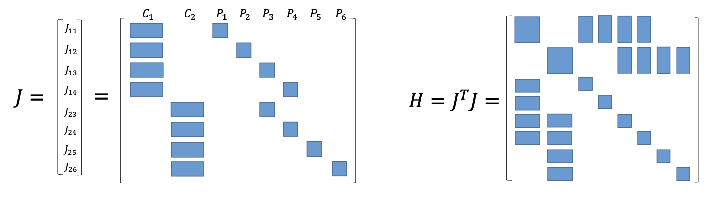
Let $H = J^T \Omega J$, $b = -J^T \Omega f(x_k)$, the matrix $H$ is an arrow-shape sparse matrix, which could be sped up by Schur complement.

$$
\begin{gather}
H \Delta x_k = b \\
\begin{bmatrix}
B & E \\
E^T & C
\end{bmatrix}
\begin{bmatrix}
\Delta x_c \\
\Delta x_p
\end{bmatrix} =
\begin{bmatrix}
v \\
w \\
\end{bmatrix}
\\
\begin{bmatrix}
B-EC^{-1}E^T & 0\\
E^T & C
\end{bmatrix}
\begin{bmatrix}
\Delta x_c \\
\Delta x_p
\end{bmatrix} =
\begin{bmatrix}
v-EC^{-1}w \\
w \\
\end{bmatrix}
\end{gather}
$$

Since matrix $C$ is an eye matrix with very large scale, $C^{-1}$ is very easy to calculate. So the $\Delta x_c$ could be solved firstly by $(B-EC^{-1}E^T)\Delta x_c=v-EC^{-1}w$, and then $\Delta x_p$ could also be solved by $\Delta x_p = C^{-1}(w - E^T \Delta x_c)$.

Accelerate In g2o library

When setting the vertex of graph optimization in g2o, there is a field called marginalized. Setting the marginalized of mappoint vertex to true and pose vertex to false could let g2o classify different vertex, then apply the Shur complement to speed up the solving.

This settings still solves all vertex, so the meaning of marginalization here is different from the meaning in sliding window scenario, which will be described in next section.

Control the Optimization Scale

As the SLAM runs, the amount of poses and mappoints turns larger and larger, especially the mappoints. In order to make sure the backend could work real-time, the scale of the optimization problem needs to be limited.

Sliding Window Optimization
Pose Graph Optimization

A sliding window could be maintained so that only up to $N$ frame/keyframes and respective mappoints will be optimized.

When removing old keyframes and respective mappoints from the sliding window, dropping them directly will lose info. Instead, the old info should be marginalized so it could become a prior term in the following optimization when new frame comes.
When adding new keyframe and new mappoints. The Jacobian of new added observation on old frame pose who was impacted by marginalized should be the same previous old Jacobian, this is called First Estimate Jacobian (FEJ), and it could guarantee the system has correct observability.

Marginalization

Old states needs to be marginalized out using Schur complement. So their info will be converted to the prior info of those states directly connected.

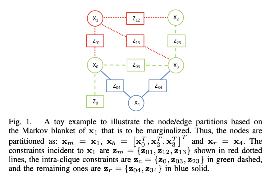
Take the above graph as an example. At the end of an optimization, we want to marginalize $x_m$, so its measurements will provide prior info for connected states $x_b$, i.e.
$$
P(x_b | z_m) = \mathcal{N}(\hat{x}_b, \Lambda_v^{-1})
$$

Then we could construct a local least square issue with $x_b, x_m, z_m$, to get
$$
\begin{split}
(\hat{x}_b, \hat{x}_m) &= \arg\max_{x_b, x_m} P(x_b, x_m | z_m) = \arg\max_{x_b, x_m} P(z_m | x_b, x_m) \\
&= \arg\min_{x_b, x_m} \sum_{i,j\in \text{span}(x_b, x_m)} \frac{1}{2} \Vert z_{ij} - h(x_i, x_j) \Vert_{\Lambda_{i,j}}
\end{split}
$$

The information matrix of joint distribution of $x_b, x_m$ are
$$
\begin{bmatrix}
\Lambda_b & \Lambda_{bm}^T \\
\Lambda_{bm} & \Lambda_m
\end{bmatrix} =
\sum_{i,j\in \text{span}(x_b, x_m)} J_{i,j}^T \Lambda_{i,j} J_{i,j}
$$
where
$$
J_{i,j} = \begin{bmatrix}
\frac{\partial e_{i,j}}{\partial x_i} \vert_{\hat{x}_i} \\
\frac{\partial e_{i,j}}{\partial x_j} \vert_{\hat{x}_j}
\end{bmatrix}
$$

Then we could get the prior of $x_b$ in the following optimization are,
$$
P(x_b) = P(x_b | z_m) = \mathcal{N}(\hat{x}_b, \Lambda_v^{-1})
$$
where

$\hat{x}_b$ is the final value of the local optimization problem
$\Lambda_v = \Lambda_b - \Lambda_{bm} \Lambda_m^{-1} \Lambda_{bm}^T$ is the Schur complement of the information matrix of the joint distribution.

Why is that?

The $H = J^T \Lambda J$ matrix constructed by Jacobian matrix provides an approximation of the Hessian matrix of the negative log-likelihood function $f(x_b, x_m) = -\log (P(x_b, x_m | z_m))$
The expectation of $H$ matrix $E_{P(x_b, x_m | z_m)}(H)$ is defined as information matrix $I$. Also the expectation could be removed since some terms in Hessian matrix is independent to $x_b, x_m$, so we have $H = I$
In Gaussian distribution, the Hessian matrix of the negative log-likelihood function $f(x_b, x_m)$ is the inverse of the covariance matrix $\Sigma$ of the distribution $P(x_b, x_m | z_m)$

Therefore, we have
$$
I \stackrel{def}{=} E(H) \approx H \approx Hessian \stackrel{Gaussian}{=} \Sigma^{-1}
$$
so we have the joint distribution
$$
P(x_b, x_m) =
\mathcal{N}(
\begin{bmatrix}
\hat{x}_b \\
\hat{x}_m
\end{bmatrix},
\begin{bmatrix}
\Sigma_b & \Sigma_{bm}^T \\
\Sigma_{bm} & \Sigma_m
\end{bmatrix}
) =
\mathcal{N}^{-1}(
\begin{bmatrix}
\eta_b \\
\eta_m
\end{bmatrix},
\begin{bmatrix}
\Lambda_b & \Lambda_{bm}^T \\
\Lambda_{bm} & \Lambda_m
\end{bmatrix}
)
$$

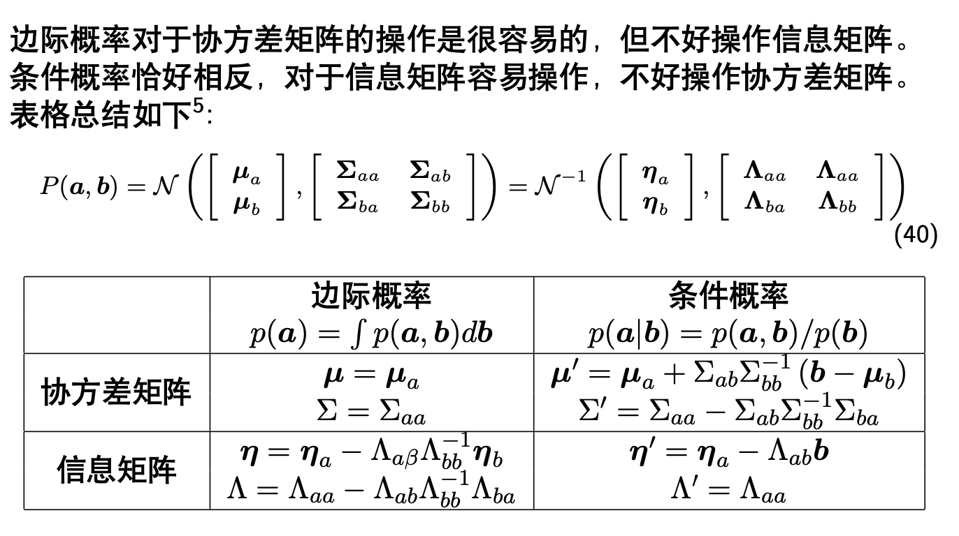
and also we have
$$
P(x_b, x_m) = P(x_m | x_b) P(x_b)
$$

Then, according to how we could decouple the joint distribution to a margin distribution and a conditional distribution.

Finally we have
$$
x_b \sim \mathcal{N} (\hat{x}_b, \Lambda_v^{-1}) = \mathcal{N} (\hat{x}_b, (\Lambda_b - \Lambda_{bm} \Lambda_m^{-1} \Lambda_{bm}^T)^{-1})
$$

In reality, in the last step of iterative when solving the local optimization problem, the left side is same as the information matrix. When we’re using the Schur complement, we actually remove the $x_m$ from $x_b$’s equations.
$$
\begin{aligned}
&\begin{bmatrix}
\Lambda_b & \Lambda_{bm}^T \\
\Lambda_{bm} & \Lambda_m
\end{bmatrix}
\begin{bmatrix}
\Delta x_b \\
\Delta x_m
\end{bmatrix} =
\begin{bmatrix}
b_b \\
b_m
\end{bmatrix} \\
\Rightarrow& \begin{bmatrix}
\Lambda_b - \Lambda_{bm} \Lambda_m^{-1} \Lambda_{bm}^T & 0 \\
\Lambda_{bm} & \Lambda_m
\end{bmatrix}
\begin{bmatrix}
\Delta x_b \\
\Delta x_m
\end{bmatrix} =
\begin{bmatrix}
b_b - b_m \Lambda_m^{-1} \Lambda_{bm}^T \\
b_m
\end{bmatrix}
\end{aligned}
$$

In summary, the Hessian matrix estimated by Jacobian matrix could provide a good approximation of the information matrix of the joint distribution, from which we could easily extract the information matrix of the margin distribution $x_b$, and use it in the following optimization as a prior.

The following optimization target turns to be
$$
x_{b,r}^* = \arg\min_{x_{b, r}} \left( \frac{1}{2} \sum_{x_b} \Vert x_b - \hat{x}_b \Vert_{\Lambda_v} + \frac{1}{2}\sum_{(i, j) \in \text{span}(x_{b, r})} e_{ij}^T \Omega_{i, j} e_{i,j} \right)
$$
where $x_b$ has both prior constraint and constraint from new observations, while $x_r$ only has constraints from new observations.

Stacking the error term together we could get
$$
f(x) = \begin{bmatrix}
x_{b0} - \hat{x}_{b0} \\
x_{b2} - \hat{x}_{b2} \\
x_{b3} - \hat{x}_{b3} \\
e_{03} \\
e_{23} \\
\vdots \\
e_{34}
\end{bmatrix},
\Omega = \begin{bmatrix}
\Lambda_v & \cdots & \cdots \\
\cdots & \Omega_{03} & \cdots \\
\cdots & \cdots & \Omega_{34}
\end{bmatrix}
$$
Then
$$
\begin{split}
J
&= \left. \frac{\mathrm{d} f(x)}{\mathrm{d} x^T} \right|_{x_k} \\
&= \begin{bmatrix}
F_{b0} & \cdots & 0 & \cdots & \cdots & 0 \\
0 & F_{b2} & 0 & \cdots & \cdots & 0 \\
\vdots & \vdots & \vdots & \vdots & \vdots & \vdots \\
\cdots & F_{ij} & \cdots & \cdots & E_{ij} & \cdots \\
\vdots & \vdots & \vdots & \vdots & \vdots & \vdots
\end{bmatrix}
\end{split}
$$
where $F_{bi} \in \mathbb{R}^{6\times 6}$ or $F_{bi} \in \mathbb{R}^{3\times 3}$ are identity matrix, depending on if $x_{bi}$ is a pose state or mappoint position state.

And the final iterative equations will be
$$
\begin{align}
J^T \Omega J
\begin{bmatrix}
\Delta x_b \\
\Delta x_r
\end{bmatrix} &=
-J^T \Omega f(x_{b, r}) \\
\left(
\begin{bmatrix}
\Lambda_v & 0 \\
0 & 0
\end{bmatrix} +
\Lambda_{b, r}
\right)
\begin{bmatrix}
\Delta x_b \\
\Delta x_r
\end{bmatrix} &=
-J^T \Omega f(x_{b, r})
\end{align}
$$

Sparsification

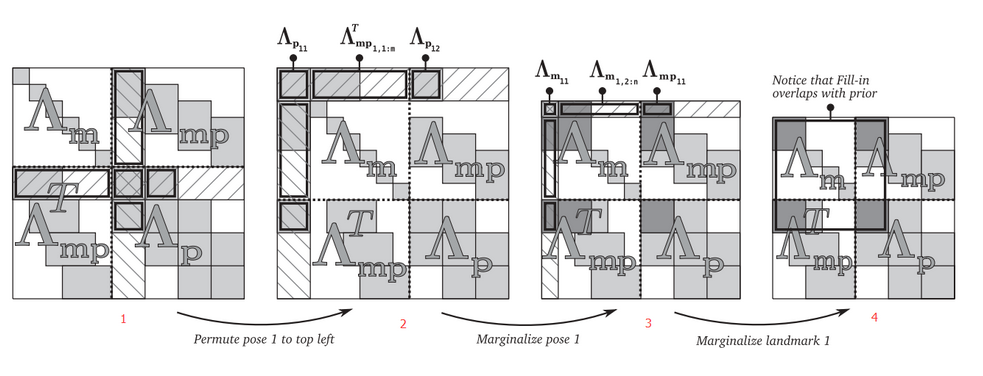
Marginalization will bring extra elements, so that the matrix $H$ is not sparse anymore. In order to maintain the sparse, following strategies could be performed.

The mappoints observed by the marginalized frame but not by other frames in the window could be marginalized
The mappoints observed by the marginalized frame but observed by other frames in the window could be removed (its observation is abandoned, influencing the accuracy but keep the optimization efficient)

Besides, in order to decrease the effect of removing mappoints. Keyframes in the window should have less common observed mappoints. The rule to select keyframes could be

The frame has large poses changed could be regarded as a keyframe
The frame with less matched keypoints with the previous frame could be regarded as a keyframe

In this way, the marginalization of old pose wouldn’t like to destroy the sparse of the matrix $H$.

Note. In some methods like ORB SLAM, the selected keyframes in the optimization have many common observations. This is to the opposite of above strategy because ORB SLAM reconstructs the whole optimization every time instead of using sliding window. It also uses other methods to include the prior information from old keyframes.

First Estimate Jacobian

To keep the consistency of the system observations, a variable can only be linearized at the same point, i.e, it’s Jacobian should be computed at the same point.

Take the above diagram as an example. After marginalization, all Jacobian of $x_2$ should take the value at $\hat{x}_2$.

Therefore, in the following optimizations, though $x_2$ will change at each iteration, the Jacobian $\frac{\partial Z_{23}}{\partial x_2}$ should always be computed at point $\hat{x}_2$. It brings more error due to linearization at a far point, but it could guarantee the observation consistency.

Since the amount of keypoints is much larger than the amount of poses, Pose Graph only keeps the poses as elements need to be optimized. In optimization graph turns to

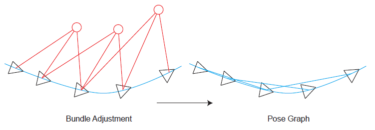
Different from the previous BA problem, where triangles are poses and circles are mappoints and the edges are errors between the pixel coordinate measurements of the keypoints $p_{ij}=[u_{ij}, v_{ij}]^T$ and the projection of space points by $h(T_{c_iw}, P_{wj})$, which is $e_{ij}=p_{ij}-h(T_{c_iw}, P_{wj})$.

The Pose Graph only considers the vertex of poses, where the edges are errors between the measurements of relative motion from frame $j$ to frame $i$, i.e. $T_{c_ic_j}$ (can be calculated by VO algorithm or by other sensors measurements like IMU) and the separate pose $T_{wc_i}, T_{wc_j}$, which are the transformation matrix of from camera at time $i$ and $j$ to world.

Therefore, the error term is defined as
$$
e_{ij}=\ln (T_{c_ic_j}^{-1} T_{wc_i}^{-1} T_{wc_j} )^{\vee}
$$

Therefore, the total error of the optimization problem is

$$\frac{1}{2}\sum_{i,j\in\epsilon}e_{ij}^T\Sigma_{ij}^{-1}e_{ij}$$
where the $\epsilon$ is the collection of all edges, and $\Sigma_{ij}$ is the information matrix.

Similar to the BA problem, the derivate of error term on $\xi_i$ and $\xi_j$ are also required, which are

$$
\begin{gather}
\frac{\partial e_{ij}}{\partial \xi_i} = -J_r^{-1}(e_{ij}) \text{Ad}(T_{c_jw}^{-1}) \\
\frac{\partial e_{ij}}{\partial \xi_j} = J_r^{-1}(e_{ij}) \text{Ad}(T_{c_jw}^{-1}) \\
\end{gather}
$$

where
$$
\mathrm{Ad}(T) = \begin{bmatrix}
R & t^{\wedge}R \\
0 & R
\end{bmatrix}
$$

Details of how to compute the derivate

Adding $\delta \xi_i, \delta \xi_j$ closed to 0 to the error term
$$
\begin{split}
\hat{e_{ij}}
&= \ln \left( T_{c_ic_j}^{-1} (\exp(\delta \xi_{i}^\wedge) T_{wc_i})^{-1} (\exp(\delta \xi_{j}^\wedge) T_{wc_j}) \right)^{\vee} \\
&= \ln \left(T_{c_ic_j}^{-1} T_{wc_i}^{-1} \exp(-\delta \xi_i^\wedge) \exp(\delta \xi_j^\wedge) T_{wc_j} \right)^{\vee}
\end{split}
$$
According to
$$
\begin{split}
& T\exp(\xi^\wedge)T^{-1} = \exp\left( (\mathrm{Ad}(T)\xi)^\wedge \right) \\
\Rightarrow & \exp(\xi^\wedge)T = T \exp\left( (\mathrm{Ad}(T^{-1})\xi)^\wedge \right)
\end{split}
$$
Then
$$
\begin{split}
\hat{e_{ij}}
&= \ln \left(T_{c_ic_j}^{-1} T_{wc_i}^{-1} \exp(-\delta \xi_i^\wedge) T_{wc_j} \exp\left( (\mathrm{Ad}(T_{wc_j}^{-1}) \delta \xi_j)^\wedge \right) \right)^{\vee} \\
&= \ln \left(T_{c_ic_j}^{-1} T_{wc_i}^{-1} T_{wc_j} \exp\left( -(\mathrm{Ad}(T_{wc_j}^{-1}) \delta \xi_i)^\wedge \right) \exp\left( (\mathrm{Ad}(T_{wc_j}^{-1}) \delta \xi_j)^\wedge \right) \right)^{\vee}
\end{split}
$$
Applying Taylor expression and only keep the linear term, then
$$
\begin{split}
\hat{e_{ij}}
&\approx \ln \left(T_{c_ic_j}^{-1} T_{wc_i}^{-1} T_{wc_j} \left( I - (\mathrm{Ad}(T_{wc_j}^{-1}) \delta \xi_i)^\wedge \right) \left( I + (\mathrm{Ad}(T_{wc_j}^{-1}) \delta \xi_j)^\wedge \right) \right)^{\vee} \\
&\approx \ln \left(T_{c_ic_j}^{-1} T_{wc_i}^{-1} T_{wc_j} \left( I - (\mathrm{Ad}(T_{wc_j}^{-1}) \delta \xi_j)^\wedge + (\mathrm{Ad}(T_{wc_j}^{-1}) \delta \xi_j)^\wedge \right) \right)^{\vee}
\end{split}
$$
According to BCH equation, when $\xi_2$ is close to 0, then
$$
\begin{split}
& \ln (\exp(\xi_1^\wedge) \exp(\xi_2^\wedge))^\vee \approx J_r^{-1}(\xi_1)^{-1}\xi_2 + \xi_1 \\
\Rightarrow & \ln (A B)^\vee \approx J_r(\ln(A)^\vee)^{-1} \ln(B)^\vee + \ln(A)^\vee
\end{split}
$$
So
$$
\begin{split}
\hat{e_{ij}}
& \approx J_r^{-1} \left( \ln(T_{c_ic_j}^{-1} T_{wc_i}^{-1} T_{wc_j})^\vee \right) \ln\left( I - (\mathrm{Ad}(T_{wc_j}^{-1}) \delta \xi_j)^\wedge + (\mathrm{Ad}(T_{wc_j}^{-1}) \delta \xi_j)^\wedge \right)^\vee + \ln \left( T_{c_ic_j}^{-1} T_{wc_i}^{-1} T_{wc_j} \right)^\vee \\
& = J_r^{-1} (e_{ij}) \ln\left( I - (\mathrm{Ad}(T_{wc_j}^{-1}) \delta \xi_j)^\wedge + (\mathrm{Ad}(T_{wc_j}^{-1}) \delta \xi_j)^\wedge \right)^\vee + e_{ij}
\end{split}
$$
Applying Taylor expression and only keep the linear term, then
$$
\begin{split}
\hat{e_{ij}}
& \approx J_r^{-1} (e_{ij}) \left( - (\mathrm{Ad}(T_{wc_j}^{-1}) \delta \xi_j)^\wedge + (\mathrm{Ad}(T_{wc_j}^{-1}) \delta \xi_j)^\wedge \right)^\vee + e_{ij} \\
& \approx J_r^{-1} (e_{ij}) \left( - \mathrm{Ad}(T_{wc_j}^{-1}) \delta \xi_j + \mathrm{Ad}(T_{wc_j}^{-1}) \delta \xi_j \right) + e_{ij} \\
& = -J_r^{-1} (e_{ij})^{-1} \mathrm{Ad}(T_{wc_j}) \delta \xi_j + J_r^{-1} (e_{ij}) \mathrm{Ad}(T_{wc_j}^{-1}) \delta \xi_j + e_{ij}
\end{split} \\
$$

Therefore,
$$
\begin{gather}
\frac{\partial e_{ij}}{\partial \xi_i} = \lim_{\delta \xi_i \rightarrow 0} \frac{\hat{e_{ij}} - e_{ij}}{\delta \xi_i} = -J_r^{-1}(e_{ij}) \text{Ad}(T_{c_jw}^{-1}) \\
\frac{\partial e_{ij}}{\partial \xi_j} = \lim_{\delta \xi_j \rightarrow 0} \frac{\hat{e_{ij}} - e_{ij}}{\delta \xi_j} = J_r^{-1}(e_{ij}) \text{Ad}(T_{c_jw}^{-1}) \\
\end{gather}
$$

Loop Closure Processing

Although frontend and backend could solve the tracking problem and limit the error to a scale, the accumulated error still exists and the drift will be very large after a period of time’s running. Loop closure detection is to detect whether the camera revisits previous areas and provide this information to the optimization.

Revisiting to a place could add an extra constraint to the optimization and this could reset the accumulated error. Besides, the techniques to check whether revisiting previous place could also be used in re-localization when the frontend tracking is lost.

Specifically, the system only includes frontend and local backend is called VO, while the frontend with local, global backend, and loop closure detection is called SLAM.

Input:
- Current image
- Previous images
Output:
- Updated frame poses if there exists loop closure
Solution:
1. Use pattern recognition to check whether revisiting previous place. e.g. bag-of-words (BoW) model
2. If found loop closure, updated the camera poses between loop image and current image
3. Merge, cull, update respective mappoints

Loop Closure Detection

Workflow

Bag-of-words (BoW) model uses a vector to describe a frame. The element in the vector represents whether there is a specific word (high-level features) appearing in the frame or how many the specific word appearing in the frame. Word in BoW model is a set of descriptors of keypoints.

The work flow using BoW model to detect the loop closure is as follows.

Generated a dictionary containing different words ahead of time. The words should have similarity with current environment
Extract the keypoints and calculates their descriptors from current frame
Check what words does current frame have from the dictionary, and generate a vector representing those words
Compare the current frame’s words vector with previous keyframes’ vectors, calculate the similarity
Determine whether there is a loop based on the similarity and additional rules
- e.g. the similarity between the loop frame and current frame should larger than the similarity between latest keyframe and current frame
- e.g. the high similarity between the loop frame with current frame should be detected several time
If the loop exists, trigger the pose and map correction steps
Store current frame’s words vector for future frames’ comparisons.

BoW Model Dictionary and Scoring

Several images with similar scenes of the running environment should be provided to generate the dictionary. The keypoints and their descriptors are extracted from each frame and they are put together to do the K-means clustering. In order to improve the check efficiency in the later steps. The dictionary could be generated into a k-ary tree shape.

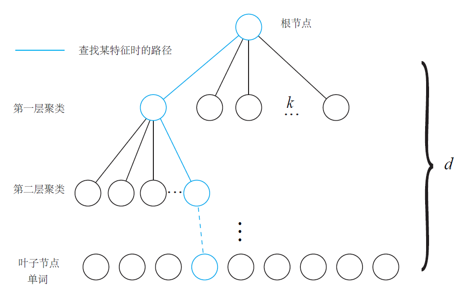
The root node contains all the descriptors extracted from several frames
In each level, split the descriptors into $k$ groups
At the final $d$ level, the descriptors in each leaf node represents a word

Therefore, a $d$ level and $k$-ary tree could have at most $k^d$ words. Each word also has a weight to describe the distinguish ability of the word. The weight could be calculated by TF-IDF (Term Frequency - Inverse Document Frequency). The weight of word $w_i$ is
$$\eta_i=\frac{m_i}{m}\log\frac{n}{n_i}$$
where

$m_i$ is the number of word $w_i$ from the detected frame
$m$ is the number of all words from the detected frame
$n_i$ is the number of descriptors in the word $w_i$ of the dictionary
and $n$ is the number of total descriptors in all words of the dictionary.

The word vector for a frame is defined as
$$ v = [v_1, v_2, \cdots, v_N]^T $$
where

$ v_i=\begin{cases}
\eta_i \quad & \text{if frame has word w_i} \\
0 \quad & \text{otherwise}
\end{cases}$
$N$ is the number of words of the dictionary

The similarity of two vectors are
$$
s(v_A, v_B) = 2\sum_{i=1}^N |v_{Ai}| + |v_{Bi}| - |v_{Ai}-v_{Bi}|
$$

Validation Loop Closure

A wrong detected loop will cause huge influence to the whole SLAM system. Therefore, the detection should be very strict although this will loses some loops. A validation part is usually added after detecting some possible loop closure. There are many means to do the validation.

Cache loops
- Store the possible loops and wait to see whether more this kind of loops could be detected
Geometric validation
- Estimate the pose change between loop frame and current frame
- Check the number of inliner and outlier points

For example

In ORB-SLAM2

Select candidates according to BoW score
1. Calculate the minimum BoW score between the current keyframe and its co-visible keyframes
2. Calculate the maximum common words between the current keyframe and its non-co-visible keyframes, set the minimum common words as 0.8 * maximum common words
3. Select the candidates from keyframes which belongs to current non-co-visible frames, and score > min BoW score, and common words > min common words
4. Iterate the candidates, put their co-visible frames together, and calculate the total score of the group. The score of its co-visible frames will be calculated only the co-visible frames belongs to the candidates
5. Calculate the maximum group score, and set minimum group score as 0.75 * max group score.
6. Select the group with score larger than minimum group score and selected the frame with largest frames from each group to form the candidate
Check the consistency of the candidate (whether it appears consistently in each time detection)
1. Iterate the candidate, create the group containing its co-visible frames
2. Check whether the group has a common keyframe with some groups of previous groups detected in last time
3. If there is a common keyframe, calculate the consistency with previous groups
4. Select the candidates whose group’s consistency larger than a threshold (3) (This means this candidate or its co-visible frames appears 3 times consistently during the detection)
Calculate Sim3 between current keyframe and each candidate and check inliner
1. Search pairs by BoW words, check the size of combination
2. Calculate Sim3, check the number of inliner
3. Use Sim3 to projects candidate’s co-visible frames’ mappoints to current maps. Check the matched number

Pose and Map Correction

Once the loop closure detection finds the loop, the poses and positions of mappoints should be corrected. The correction could also happens in backend with BA method. But usually the loop closure detection has its own thread to preform the correction.

Generally, the pose change $T_{c_ic_j}$ between the current keyframe and the loop-frame could be calculated by VO method. This could forms a pose graph optimization problem.

For example

In ORB-SLAM2

Calculate the relative pose from loop-frame to current frame $T_{cl}$
Use the pose of loop-frame and relative pose to correct the pose of current frame $T_{cw} = T_{cl}T_{lw}$. Then corrects the position of its observed mappoints
Use the relative pose between the current frame and its co-visible frames $T_{ic}$ to correct its co-visible frames poses $T_{c_iw}=T_{ic}T_{cw}$. Then corrects the position of each co-visible frames’ mappoints
Fuses the mappoints from loop frames’ co-visible frames and current frames’ co-visible frames
Get the new added co-visible relationships of each current frame since new mappoints are added
Optimize the Essential Graph, which is the pose graph where edges come from
- Measurement is corrected poses
  - new added co-visible relationships.
- Measurement is before-corrected poses
  - each keyframe with its father keyframe.
  - previous loop relationships.
  - previous co-visible relationships with high weight
Start a new thread to perform global BA for all keyframes and mappoints

Mapping

SLAM mainly focuses on localization instead of mapping, where the efficiency and realtime is emphasized.

Map Management

Map Management is the mechanism to manage reconstructed map in backend, serving to frontend to improve the tracking accuracy. Specifically, a SLAM system needs to consider

When to add new mappoint to map
When to remove existing mappoint from map (map prune)
How to marginalize the mappoint
How to determine whether a mappoint position needs to be optimized
How to optimize the mappoint position in map
What submap serves to frontend for tracking

Since backend map is usually constructed from keyframes, which will be also stored in the map, so there are more considerations

When to accept new keyframe
How to extract new mappoints from new keyframe
How to optimize the both the new and existing mappoint positions with keyframe poses
When to remove existing keyframes (map prune)
How to marginalization keyframes and mappoints
How to present the mappoint position (3D or inverse depth)

3D Reconstruction

The reconstructed map from SLAM frontend and backend, which is a 3D point cloud, represents the sparse features of the space. The sparse map only contains several space points and cannot describe the details of the environment like surface or different objects. Sparse map could benefit the localization but cannot handle complex tasks like plane ray-casting in AR, navigation of autonomous vehicles.

Therefore, different kinds of map could be constructed based on the captured images and camera pose calculated from frontend and backend. Map could have different categories like metrics map, which describes the details of the environment and topological map, which focuses the connectivity among elements. Below are different kinds of metrics maps and their using scenarios.

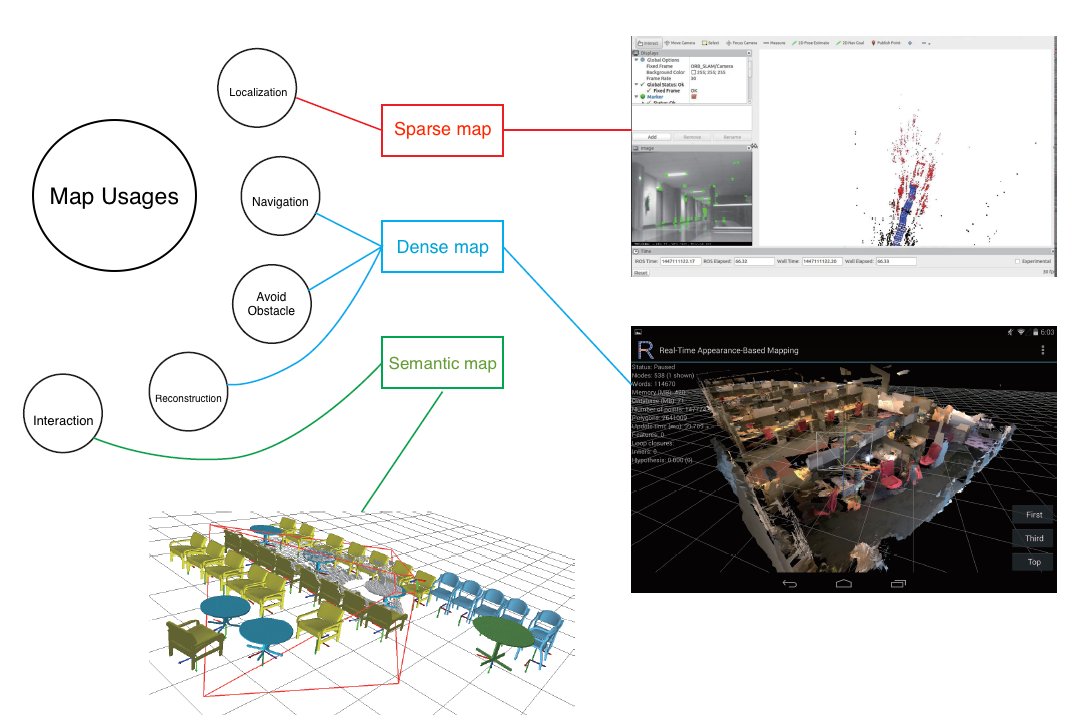
Semantic map requires deep learning techniques to identify the objects, thus the sparse map and dense map are explained here.

Aspects	Spare map	Dense map
What is it	3D point cloud calculated from SLAM frontend and backend	3D point cloud containing more points, usually not come from realtime SLAM system
Point data	$(Gray, X, Y, Z)$ or $(R, G, B, X, Y, Z)$ to describe their color and position in world system	same
Point type	Mappoints of those matched keypoints. Scatter point in space	Mappoints of all pixels of the frames. To limit the redundant information. A cube area in space only contains 1 mappoint. The size of the cube is the division value of the map

Dense Map

Build map with different sensors

If the visual camera is RGB-D camera, the depth of space point corresponding to each pixel could be directly measured. Then the dense map could be established from different frames and their camera poses. Filter will be adopted in the end to remove redundant information

If the visual camera is monocular or stereo camera, the depth of space point needs to be calculated by triangulation of matched keypoints. However, not all the pixels in the images are special enough to be keypoint, thus finding their respective keypoint in another image requires the epipolar search.

Epipolar search

Input
- 2-d pixel $p_1 = [u_1, v_1]^T$ in first image’s pixel frame
- Relative pose $T_{c_2c_1}$
Output
- Respective pixel $p_2 = [u_2, v_2]^T$ in second image’s pixel frame
Solution
- Need to search along the line $l_2 = F\mathbf{p}_1$ in image 2 to find the most similar pixel patch

$$
\begin{split}
&\mathbf{p}_2^T F \mathbf{p}_1 = \mathbf{p}_2^T K^{-T} t_{c_2c_1}^\wedge R_{c_2c_1} K^{-1} \mathbf{p}_1 = 0 \\
\Rightarrow& (F\mathbf{p}_1)^T \mathbf{p}_2 = 0 \\
\Rightarrow& (F^T\mathbf{p}_2)^T \mathbf{p}_1 = 0
\end{split}
$$

Post-processing of map

The dense map is still 3D point cloud, so it’s still not enough to support complex using scenarios like AR or navigation. Therefore, some techniques need to be applied on the dense map to generate more details.

Mesh, surfel for rendering map
- Build the surface among points
Voxel for occupancy map
- Divide the map into voxels (usually is cubes) on a resolution
- Each voxel has 3 status: occupied, free, and unknown. Use a float ${0, 1}$ to describe the status
- This occupancy map could be used for navigation
- Could used octomap to reduce the size of the occupancy map

Bowen's Tech Blog

Visual SLAM Introduction

Glossary

Categories of Visual Sensors

Camera Basis

Frontend

Feature-based Method

2D-2D: Epipolar Constraint

Triangulation

3D-2D: PnP

3D-3D: ICP

Direct Method

Backend

Filter Method

Optimization Method

Build Optimization Target (Cost Function)

Solve the Least Square Problem

Control the Optimization Scale

Loop Closure Processing

Loop Closure Detection

Workflow

BoW Model Dictionary and Scoring

Validation Loop Closure

Pose and Map Correction

Mapping

Map Management

3D Reconstruction

Dense Map

Reference