Advanced SLAM Literature Review
Literature review for SLAM papers that use neural network / deep learning based approaches.
Individual Task
Data Association
SuperPoint: Self-Supervised Interest Point Detection and Description
Extract feature points with DNN model
- Generating synthetic dataset with basic shapes and known corner points
- Train MagicPoint model (base model)
- Soft labeling real dataset with Homography Adaption
- Train final SuperPoint model (final model)
SuperPoint model consists of 1 encoder, 1 decoder providing the probability as a keypoint for each pixel, and 1 decoder providing descriptor for each pixel.
SuperGlue: Learning Feature Matching with Graph Neural Networks
Match two sets of keypoints + descriptors (e.g. from SuperPoint) between an image pair with a GNN model.
- Keypoint encoder: each keypoint’s position and detection confidence is embedded by an MLP and added to its visual descriptor, giving every keypoint a combined position + appearance representation
- Attentional Graph Neural Network: alternates self-attention (within the same image, to encode spatial relationships between own keypoints) and cross-attention (against the other image, to compare appearance and enable early rejection/agreement) across multiple layers to enrich the keypoint representations with context from both images
- Optimal matching layer: computes a score matrix from the inner product of the final descriptors, then augments it with a learned “dustbin” row/column so keypoints with no valid correspondence (occlusion, non-overlap) can be explicitly assigned to “no match”
- The augmented score matrix is solved as a differentiable optimal transport problem via the Sinkhorn algorithm, producing a soft partial assignment matrix that is supervised end-to-end against ground-truth matches derived from known poses/depth
Bundle Adjustment
BA-Net: Dense Bundle Adjustment Networks
Solves dense SfM (structure + pose) by making Bundle Adjustment itself part of the network, rather than treating it as a separate post-processing optimization step.
- Depth parameterization: rather than optimizing every pixel’s depth independently, a CNN predicts a small set of per-image basis depth maps; the final dense depth is a linear combination of these bases, so BA only has to solve for a handful of combination weights per image plus the camera poses
- Feature-metric BA: instead of the classic photometric error, the residual is the difference between learned deep feature maps of the two views at corresponding reprojected points — features are trained to make this error surface smoother and less prone to bad local minima
- Differentiable Levenberg-Marquardt (LM): a small network predicts the LM damping factor at each optimization iteration (rather than hand-tuning it), so the entire iterative optimization loop is differentiable end-to-end. Depth bases, features, and the damping-factor network are all trained jointly by backpropagating through the unrolled LM iterations against ground-truth pose/depth
- Net effect: combines hard-coded multi-view geometry constraints (the BA cost function and LM update rule are still classic geometry) with learned components (features, depth bases, damping) — geometry stays interpretable while the error landscape it optimizes becomes learned
Note of differentiable optimization
Differentiable optimization is not a “learned optimizer” which directly estimates the final results of the least square question with neural network. Instead, it’s still the classic optimization solver but with backpropagate path after solving the question.
Differentiable optimization needs to calculate the derivate of final optimization result over the parameters of the optimization target $\frac{\partial x^\star}{\partial \theta}$, where
$$
x^\star = \arg\min_x E(x, \theta)
$$
which could be solved by chain of each optimization step or leverage the fact $\nabla_x E(x^\star, \theta) = 0$
This could enable the neural network in frontend which predicts feature correspondence or other parameters to learn from optimizing the trajectory error instead of just focusing on feature matching correct rate.
Backend Map Representation
iMAP: Implicit Mapping and Positioning in Real-Time
Shows that a single small MLP can be the entire map — replacing landmarks, voxels, or point clouds.
- Map representation: one MLP $F_\theta(x) \rightarrow (\text{occupancy}, \text{color})$ maps a 3D coordinate directly to occupancy probability and color, analogous to NeRF’s density+color field but trained live, incrementally, per-scene
- Rendering/tracking: a depth and color image can be rendered from any candidate camera pose by ray-marching through the MLP (as in NeRF); tracking a new frame is done by holding the MLP fixed and optimizing only the camera pose to minimize photometric + depth rendering error against the observed frame
- Mapping is joint keyframe bundle adjustment, but over network weights: a small set of selected keyframes’ poses and the MLP weights are jointly optimized together (instead of adjusting explicit landmark positions, as in classic BA, you adjust the implicit function that generates them)
- Efficiency tricks needed to hit real-time: information-guided pixel sampling (spend rendering/optimization budget on pixels with high current loss, i.e. poorly-explained regions, rather than uniformly), and sparse keyframe selection based on expected information gain, so mapping doesn’t have to replay every frame ever seen
- Side benefit of the implicit representation: unobserved regions (e.g. the back of an object) are automatically filled in smoothly and plausibly by the MLP’s inductive bias, rather than left as holes as in explicit point/voxel maps
NICE-SLAM: Neural Implicit Scalable Encoding for SLAM
Addresses iMAP’s two main weaknesses — a single global MLP over-smooths detail and doesn’t scale to large scenes, since it has to compress the entire scene into one small network — by moving from “one MLP is the whole map” to “one grid of local features is the map”.
- Hierarchical feature grids: instead of one implicit function for the whole scene, geometry is stored in multiple resolutions of an explicit voxel feature grid (coarse/mid/fine), each holding a small learnable feature vector per voxel; querying a 3D point interpolates nearby voxel features at each level
- Frozen, pretrained MLP decoders turn the interpolated multi-resolution features into occupancy/color at query time, so — unlike iMAP, which trains its MLP live from nothing — only the feature grids (and periodically, keyframe poses) are optimized online; the decoders themselves are fixed after pretraining
- Because each 3D point only touches a handful of nearby voxels, tracking/mapping updates only need to backpropagate into the local grid cells actually seen by the current frame — a sparse update, unlike iMAP’s single MLP where every training step touches the entire (shared, global) set of weights. This locality is what lets it scale to room- and building-sized scenes without the fine detail all collapsing to one shared low-capacity network
- Tracking and mapping otherwise follow the same pattern as iMAP: render depth/color by ray-marching against the current representation, optimize pose against a fixed map for tracking, and jointly optimize the map (here, grid features) with a window of keyframe poses for mapping
Whole Architecture
DROID-SLAM: Deep Visual SLAM for Monocular, Stereo, and RGB-D Cameras
Deep-learning based SLAM system built around a recurrent, iterative update operator that refines camera poses and per-pixel depth, combined with a differentiable Dense Bundle Adjustment (DBA) layer.
The frontend and backend reuse the exact same update operator + DBA layer, just applied to different scopes of the frame graph.
- Frontend (per-frame tracking, real time)
- Feature extraction: two CNNs (a feature network and a context network) encode each incoming frame into dense feature maps at 1/8 resolution
- Frame graph: a co-visibility graph over a sliding window of recent keyframes; edges connect frames with shared view overlap and are added/dropped dynamically as new keyframes come in, based on mean optical flow between frames
- Correlation pyramid: for every edge in the local frame graph, dot-product all pairs of pixel features between the two frames to build a 4D correlation volume, then average-pool it at multiple resolutions so the update operator can later look up correlation features at different search radii
- Update operator (ConvGRU, applied iteratively like RAFT): takes the current pose/depth estimate (as induced optical flow), correlation features looked up around that flow, the hidden state, and context features, and outputs a revision to the flow field plus a per-pixel confidence weight each iteration
- Local Dense Bundle Adjustment: treats the predicted flow revision as a target 2D correspondence and solves a Gauss-Newton step over just the local frame graph, weighted by the predicted confidence
- Keyframe selection: new frames are promoted to keyframes based on optical-flow magnitude relative to the latest keyframe
- Backend (global consistency, runs periodically)
- Reuses the identical update operator + DBA layer from the frontend, but runs it over the entire accumulated frame graph rather than just the local sliding window
- Loop closure: extra edges are added between keyframes that are spatially close but not temporally adjacent, letting the same DBA machinery correct accumulated drift — no separate loop-closure network is needed
- Periodically performs global BA over the whole trajectory of keyframes, jointly refining all poses and per-pixel depths
- Training: end-to-end on monocular video (TartanAir), unrolling many update/DBA iterations per training example and supervising pose and flow at each iteration, similar to RAFT’s training scheme
- Because the DBA layer’s cost term only assumes per-pixel correspondence, the same monocular-trained network can be applied to stereo or RGB-D input at test time by fixing/constraining depth with the extra sensor data, without retraining
SLAM3R: Real-Time Dense Scene Reconstruction from Monocular RGB Videos
Proposed deep-learning based method to perform 3D reconstruction from video sequence without estimating frame poses and camera parameters
- Middle frame from the clip will be treated as keyframe
- I2P (Image to Points) model: output 3D points from a video clip (a sliding window of original video)
- multi-branch ViT (Visual Transformer)
- Input: frames from a clip with 1 frame as keyframe
- Output: features of each frame, 3D points reconstructed and their confidence
- Model structure
- Encoder: encode each frame from the clip to features
- Keyframe Decoder: self-attention for keyframe features, cross-attention for keyframe features v.s. all supporting frames’ features
- Supporting Decoder: cross-attention for each supporting frame’s features v.s keyframe features
- Buffering set
- Hold up to
Bregistered frames / scene frames for global reconstruction - When a new keyframe after I2P, it may be treated as a scene frame. If chosen as scene frame, it will be inserted into buffering set and replace one of the current frame
- When a new scene keyframe comes, its features will be fed into a retrieval model to compute correlation score v.s. each of other scene frame in the buffering set. The top-
Kbest-correlated keyframes will be selected as global reference to fuse the current scene keyframe
- Hold up to
- L2W (Local to World) model: incrementally register local point clouds to the global point cloud
- Input: K scene frames and a new keyframes with their features and 3D points from I2P
- Output: new (transformed) 3D points in global reference frame
- Model structure
- Points embedding: encode 3D points from each scene frame into (geometric) features. Combine with visual features from I2P for each scene frame
- Registration decoder: self-attention for keyframe features (visual + geometric), cross-attention for keyframe features v.s. all scene features
- Scene decoder: cross-attention for each scene features v.s. keyframe features
SLAM-Former: Putting SLAM into One Transformer
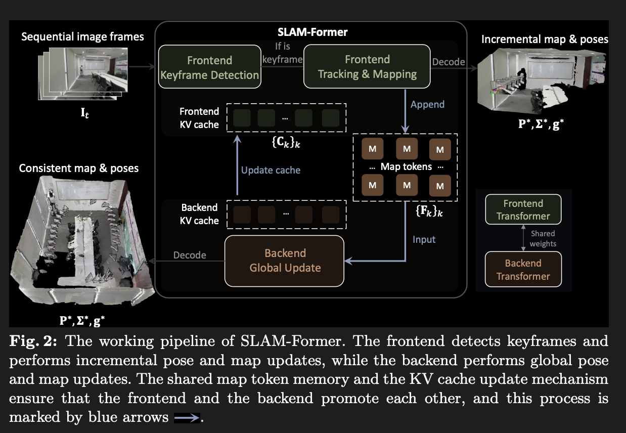
SLAM-Former fully depends on neural network. It consists of a frontend and a backend module, while they rely on the same transformer backbone with different heads.
- Architecture
- Frontend
- Input: image tokens of camera frame, updated KV caches of previous frames from backend
- Output: map tokens, could be decode into mappoints, confidence and poses with different heads
- Steps
- Decide if the new frame is a keyframe by inference the new frame against latest keyframe’s KV cache through the transformer and the pose head, and check if the relative pose exceed threshold. Only keyframe will be processed for following steps.
- Rerun the inference of current keyframe against the full KV caches frontend maintains to get map tokens
- Store the current keyframe’s KV cache for next frame’s processing
- Backend
- Input: map tokens from frontend
- Output: refined map tokens, and respective KV caches for frontend
- Steps:
- After every T keyframes, run the inference with accumulated map tokens from frontend to refine the map.
- Share the resulting KV caches to frontend. So that frontend tracks new frames against refined maps.
- Frontend
- Training
- Model structure: 36 transformer layers
- 3 training modes
- Causal attention: Only takes in images tokens, for frontend inference with accumulated KV caches.
- Mixed attention: Takes in both images and map tokens, for frontend inference with mixed KV caches from backend and frontend
- Full attention: Only takes in map tokens, for backend inference
- Loss
- Depth loss: the loss for recovered depth frames
- Point map loss: the loss for local point map
- Pose loss: the loss of relative pose changes
Note. “attend to cached K/V from tokens X” and “concatenate X as literal input tokens and run the full forward pass” produce bit-identical outputs for the new tokens.