SLAM Learning Resources
This post organizes the resources that I used to learn SLAM, also serves as a reference to other post in this blog.
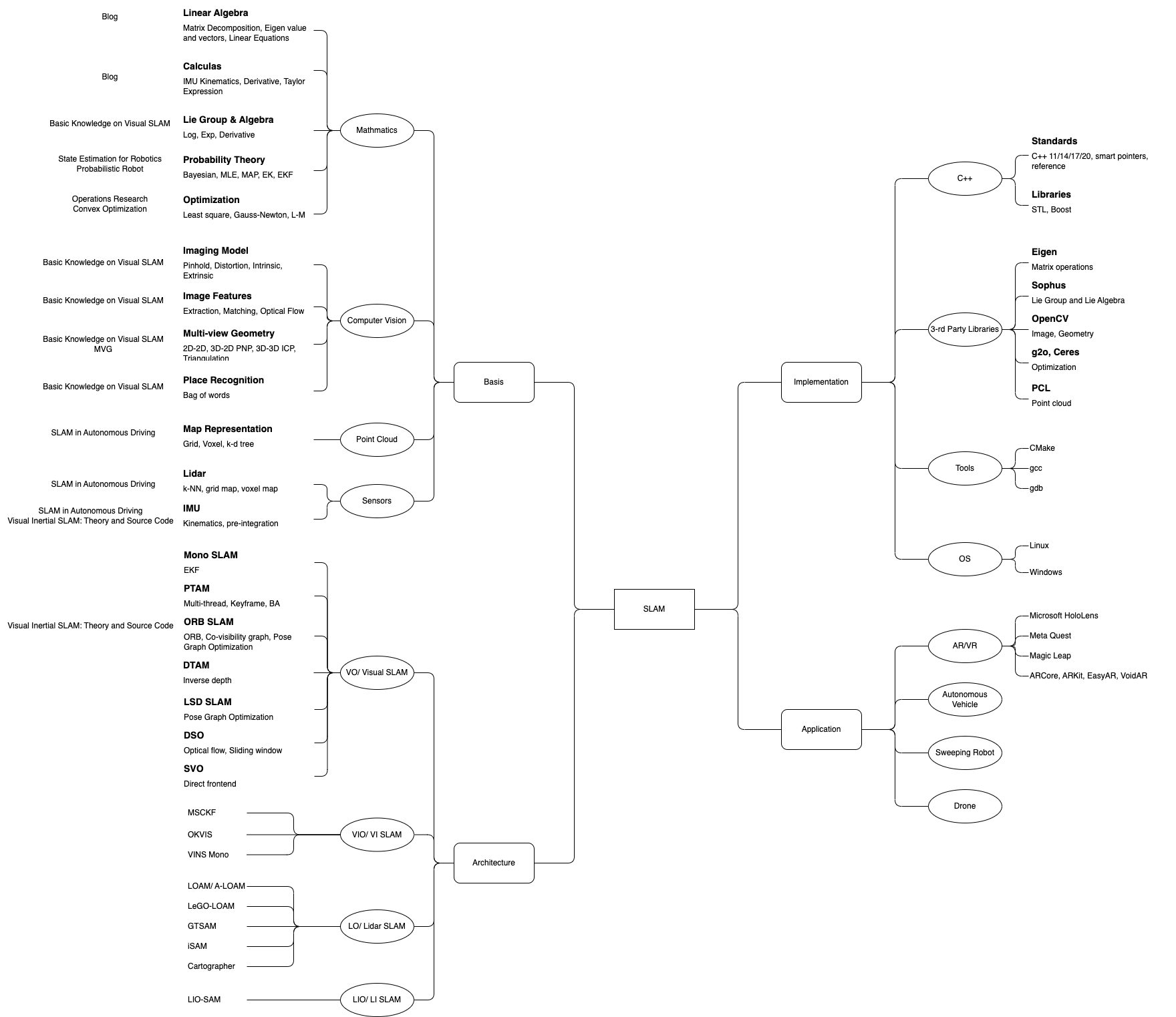
SLAM Knowledge Graph
Book
| English Version | Chinese Version | Description |
|---|---|---|
| Basic Knowledge on Visual SLAM: From Theory to Practice | 视觉SLAM十四讲 | Visual SLAM architecture, including frontend, backend, loop closing detection, mapping, Lie Group and Lie Algebra and optimization |
| SLAM in Autonomous Driving book | 自动驾驶中的SLAM技术 | IMU Kinematics, pre-integration, ESKF, IEKF, GINS, LO, Loosely-coupled / Tightly-coupled LIO, High-fi map |
| Visual Inertial SLAM: Theory and Source Code | 视觉惯性SLAM:理论与源码解析 | SLAM engineering details based on ORB SLAM 2 & 3. VIO, multi-map theory |
| State Estimation for Robotics | 机器人学的状态估计 | SLAM backend mathematic theory. Recursive methods and batch estimations methods for MAP estimation. Lie Group and Lie Algebra for 3D space optimization |
| Multiple View Geometry in Computer Vision | 计算机视图中的多视图几何 | 2D/3D Euclidean/Projective Transformations, Camera projection model, monocular, 2-view, 3-view and multi-view geometry |
| Convex Optimization | 凸优化 | Methods to analyze and solve optimization problem |
| OpenCV related books | ~ | Some books focus on the application of OpenCV like AR, SfM, Object Detection |
Course
| Course Name | Description |
|---|---|
| Online Lectures: Basics for Robotics & Photogrammetric Computer Vision (Cyrill Stachniss, 2020) | Introduces the 3d space movement and basic Mathematics theory used in SLAM like homogeneous coordinates, RANSAC |
| Online Course: Photogrammetric Computer Vision Block - Course Introduction (Cyrill Stachniss, 2020) | Covers the details about different CV algorithm, including feature extraction and pose calculation from images |
| 运筹学相关课程 | Covers lots of content, but could only focus on how to solve non-linear optimization problem for learning |
Classic Paper
- For visual SLAM, refer to this blog
- For visual inertial SLAM, refer to this blog
- Unified Inverse Depth Parametrization for Monocular SLAM
Related Paper
Blogs
Knowledge Index
Describe camera pose in space
- Pose change matrix $T$
- SO(3), SE(3), so(3), se(3)
- Homogeneous coordinate
- Different projection types
- 3D - in homogeneous coordinate
- Euclidean: rotation + translation, 6DoF
- Similarity: rotation + translation + scale: 7DoF
- Affine: 12DoF
- Projective: 15DoF

- 2D - in homogeneous coordinate
- Rigid / Euclidean: rotation + translation, 3DoF
- Linear: rotation + scale, 2DoF
- Similarity: rotation + translation + scale, 4DoF
- Affine: rotation + translation + scale + shear, 6DoF
- Projective: 8DoF
- 3D - in homogeneous coordinate
Camera imaging model
- Pinhole camera model
- Focal length x, y, optical center, skew coefficient, all in pixels
- Coordinate in camera frame, normalized imaging plane, pixel frame
- Lens distortion
- radial distortion, tangential distortion
- Calibration - Zhang’s method
Frontend - Feature-based method
- Feature extraction
- Keypoints and descriptors
- ORB feature (Oriented FAST and Steer BRIEF)
- Feature matching
- Brute force
- FLANN (Fast library of approximate nearest neighbors)
- Optical flow
- Pixel patch
- 2D-2D
- Fundamental and essential matrix (vector in same plane)
- 8 point pairs, 8 unknown
- Singular value $(\sigma, \sigma, 0)^T$
- Recover $R$ and $t$ from $E$
- Homography matrix (pixels relationship assuming there are in same plane)
- 4 point pairs, 8 unknown
- Triangulation
- Fundamental and essential matrix (vector in same plane)
- 3D-2D
- DLT
- 6 point pairs, 12 unknown
- P3P
- 3 points + 1 point for validation
- Bundle adjustment (similar to backend)
- DLT
- 3D-3D
- ICP, SVD
- Bundle adjustment (similar to backend)
Frontend - Direct method
- Minimizing photometric error
- Similar to backend optimization
Backend - Filter (MAP, Incremental)
- Kalman filter
- Extended Kalman filter
Backend - Optimization (Usually MLE, Batch)
- Optimization target
- Put poses and mappoints together as the state vector
- Derivate of error term on pose
- Derivate of error term on mappoint’s position
$$
\frac{\partial e_{ij}}{\partial \xi_i} = -\left[\begin{matrix}
\frac{f_x}{Z_j^{\prime}} & 0 & -\frac{f_x X_j^{\prime}}{(Z_j^{\prime})^2} & -\frac{f_x X_j^{\prime} Y_j^{\prime}}{(Z_j^{\prime})^2} & f_x+\frac{f_x(X_j^{\prime})^2}{(Z_j^{\prime})^2} & -\frac{f_x Y_j^{\prime}}{Z_j^{\prime}} \\
0 & \frac{f_y}{Z_j^{\prime}} & -\frac{f_y Y_j^{\prime}}{(Z_j^{\prime})^2} & -f_y - \frac{f_y(Y_j^{\prime})^2}{(Z_j^{\prime})^2} & \frac{f_y X_j^{\prime} Y_j^{\prime}}{(Z_j^{\prime})^2} & \frac{f_y X_j^{\prime}}{Z_j^{\prime}}
\end{matrix}\right]
$$
$$
\frac{\partial e_{ij}}{\partial p_j} = -\left[\begin{matrix}
\frac{f_x}{Z_j^{\prime}} & 0 & -\frac{f_x X_j^{\prime}}{(Z_j^{\prime})^2} \\
0 & \frac{f_y}{Z_j^{\prime}} & -\frac{f_y Y_j^{\prime}}{(Z_j^{\prime})^2}
\end{matrix}\right] R_i
$$
- Solve delta element $\mathbf{H} \mathbf{\Delta x} + \mathbf{b} = 0$
- Schur complement
- Iterative solution
- Gradient Descent - first derivate of $F(\mathbf{x})$
- Newton - second derivate of $F(\mathbf{x})$
- Gauss-Newton - first derivate of $f(\mathbf{x})$
- Levengerg-Marquardt - combination of gradient descent and gauss-newton
- Acceleration
- Sliding window
- Marginalization using Schur complement
- Pose graph
Loop Closure
- Use K-means to build the dictionary, which is a d level k-ary tree
- Use vector to represent the words frequency appearing in the frame